| Issue |
Wuhan Univ. J. Nat. Sci.
Volume 31, Number 2, April 2026
|
|
|---|---|---|
| Page(s) | 112 - 120 | |
| DOI | https://doi.org/10.1051/wujns/2026312112 | |
| Published online | 13 May 2026 | |
Aquatic Ecology and Water Environment Safety
CLC number: O175.13
Global Stability of Aquatic Ecosystems with Terrestrial Organic Carbon
具有陆地有机碳输入的水生生态系统全局稳定性
School of Mathematics and Statistics, Weinan Normal University, Weinan 714099, Shaanxi, China
(渭南师范学院 数学与统计学院, 陕西 渭南 714099)
Received:
2
May
2025
Abstract
To quantitatively analyze the physical and biological dynamics of terrestrial organic carbon (TOC), phytoplankton, and zooplankton, and to clarify the relationship between global stability and the input TOC concentration, this paper proposes a mathematical model for aquatic ecosystems. The interactive dynamics are analyzed by using Hurwitz’s criterion, LaSalle’s invariance principle, and appropriate Lyapunov functions. Key results show that the phytoplankton-free equilibrium is globally asymptotically stable at high input TOC concentrations. In contrast, the coexisting equilibrium exhibits global asymptotic stability under low input TOC conditions. These theoretical findings are validated by numerical simulations, highlighting the importance of monitoring and regulating input TOC concentrations to preserve biodiversity.
摘要
为定量解析陆地有机碳(TOC)、浮游植物与浮游动物的动力学过程,揭示平衡点的全局稳定性与TOC输入浓度的内在关联,本文构建了水生生态系统的数学模型。借助Hurwitz判据、LaSalle不变性原理及适配的Lyapunov函数,系统地分析了模型的交互动力学特性。研究发现:当TOC输入浓度处于较高水平时,无浮游植物平衡点呈现全局渐近稳定性;而在低浓度TOC输入条件下,系统共存平衡点表现出全局渐近稳定性。数值模拟结果进一步验证了理论结论,明确了监测与调控TOC输入浓度对维系水生生物多样性的关键意义。
Key words: terrestrial organic carbon / Holling type Ⅱ functional response / equilibrium / stability analysis
关键字 : 陆地有机碳 / Holling Ⅱ 型功能反应 / 平衡点 / 稳定性分析
Cite this article:XUE Chunrong. Global Stability of Aquatic Ecosystems with Terrestrial Organic Carbon[J]. Wuhan Univ J of Nat Sci, 2026, 31(2): 112-120.
Biography: XUE Chunrong, female, Associate professor, research direction: biological mathematical model. E-mail: This email address is being protected from spambots. You need JavaScript enabled to view it.
Foundation item: Supported by the Natural Science Foundation of Shaanxi Province (2022JZ-09)
© Wuhan University 2026
 This is an Open Access article distributed under the terms of the Creative Commons Attribution License (https://creativecommons.org/licenses/by/4.0), which permits unrestricted use, distribution, and reproduction in any medium, provided the original work is properly cited.
0 Introduction
Zooplankton have a significant impact on the structure and function of the lake ecosystem by acting as both predators of bacteria and phytoplankton and prey for fish. The primary energy source for zooplankton is believed to be organic carbon derived mainly from endogenous sources within the lake. However, advancements in stable isotope technology have demonstrated that carbon within aquatic food webs also originates from external inputs such as terrestrial organic carbon (TOC)[1-2]. Recent studies indicate that external sources, including terrestrial dissolved organic carbon (T-DOC), terrestrial particulate organic carbon (T-POC), and terrestrial prey (T-prey), along with surface runoff and other pathways, significantly contribute to allochthonous carbon in lakes[3-4]. Research has focused on how zooplankton acquire and utilize TOC[4-6]. Findings from previous studies suggest that TOC plays a vital role in supporting zooplankton growth and reproduction[7-9]. Additionally, studies suggest that TOC may account for 22% to 75% of zooplankton diets in nutrient-poor lakes[10]. Zooplankton acquire these subsidies by consuming organic detritus and feeding on heterotrophic bacteria that feed on TOC[11-13].
Due to the challenges of measuring plankton biomass directly, mathematical models are essential for understanding the physical and biological dynamics of plankton ecosystems[14-15]. Previous research has primarily focused on zooplankton-phytoplankton systems, emphasizing dynamic behavior, equilibrium point stability, Hopf branches, global stability assessments, and global Hopf branches[16-20]. In the context of the Three Gorges Reservoir area, a novel nutrient-plankton dynamics model was developed to explore the relationship between global stability and nutrients. The findings revealed that environmental pollution, nutrient cycling, and overfishing have the potential to affect water quality and the collapse of aquatic ecosystems[21]. Furthermore, Zhang and Wang[22] introduced Holling type I functional responses for phytoplankton-nutrient interactions and Holling type Ⅱ for phytoplankton-zooplankton interactions. Their analysis of the model’s global bifurcation and equilibrium point stability revealed that phytoplankton blooms can occur even at low nutrient input rates.
TOC plays a significant role in sustaining the planktonic food web in lakes and is essential for consumer nutrition. However, research on plankton systems with TOC remains limited. Inspired by reviews in Refs. [23-24], we propose a model of the carbon-phytoplankton-zooplankton (CPZ) system, which includes TOC, phytoplankton (P), and zooplankton (Z). The development of this CPZ dynamical system will enhance the understanding of planktonic ecosystem interactions. Through the analysis in this study, we aim to gain valuable insights into the overall functioning of aquatic ecosystems. Ultimately, this research seeks to contribute to a more comprehensive understanding of how TOC maintains stability in aquatic systems.
The paper is structured as follows. Section 1 formulates the CPZ model and presents two key theorems: one establishing the existence of a positive invariant set that guarantees nonnegative solutions, and another proving the existence of equilibrium points under biologically feasible parameter conditions. And then three theorems are rigorously established in Section 2 to characterize the instability of the plankton-free equilibrium and the global asymptotic stability of both the phytoplankton-free equilibrium and the coexistence equilibrium. Section 3 presents selected numerical simulations to validate the theoretical analyses and illustrate the dynamical behaviors of the CPZ model. Finally, Section 4 concludes the paper with a brief discussion.
1 CPZ Model with TOC
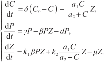
The CPZ dynamical model with Holling type Ⅱ functional responses for TOC-zooplankton interactions can be characterized by the following differential system:
 (1)
(1)
For simplicity, we only consider TOC, phytoplankton, and zooplankton in the aquatic system. Let  represent the concentration of TOC available for zooplankton uptake at time
  , while
  and
and  denote the densities of phytoplankton and zooplankton, respectively. The parameter
  is the dilution rate, and
  is the constant input concentration of TOC. Parameters
  and
and  denote the maximum specific uptake rate and half-saturation constant of zooplankton, respectively. Additionally,
  denotes the intrinsic growth rate of phytoplankton, whereas
  represents their death rate. It is reasonable to assume that
  . The parameter
  describes the predation coefficient of zooplankton, while parameters
  and
and  represent the conversion rates from phytoplankton to zooplankton and from TOC to zooplankton respectively. Finally,
  indicates the death rate of zooplankton. All parameters are assumed to be nonnegative.
In a biological framework, the densities of phytoplankton and zooplankton are nonnegative for all  . Similarly, the input concentration of TOC remains nonnegative for all
  . Consequently, system (1) is governed by the following initial conditions,
 (2)
(2)
Next, we mainly focus on the positively invariant region of the CPZ dynamical system, which underpins the existence of several equilibria.
Theorem 1 The set 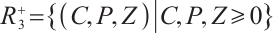 is a positively invariant region for system (1).
Proof When  , the first equation of (1) reduces to
  , it implies
 (3)
(3)
Integrating both sides of the last two equations of (1) with respect to  , we obtain the expressions for
  and
and  , where
 (4)
(4)
Using the initial value conditions (2)-(4), it is evident that  hold for all
  . This confirms that
 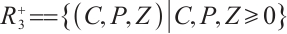 is indeed the positively invariant region for system (1).
The study subsequently focuses on positive constant equilibrium solutions of system (1), which are derived through the solution of the following algebraic equation system,
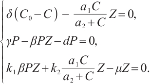 (5)
(5)
The solution to the third equation of (5) yields  or
or
 (6)
(6)
Similarly, the second equation of (5) implies in  or
or
 (7)
(7)
When  , solving the first two equations of (5) yields
  , and
, and  .
.
Therefore, the plankton-free equilibrium  always exists. This equilibrium corresponds to a state in which only TOC persists, with no viable plankton populations.
Next, we turn to analyzing interior equilibria, which require solving the full system of the algebraic equations (5).
The third equation of (5) can be rewritten as
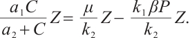
Substituting the left-hand side expression with its right-hand side into the first equation of (5), we derive the following algebraic equation:
 (8)
(8)
When  , the solutions to equations (6) and (8) are given by
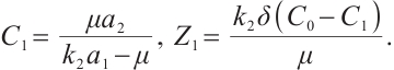 (9)
(9)
Consequently, when  and
and  , the phytoplankton-free equilibrium
  exists, which involves TOC and zooplankton. This equilibrium characterizes a stable state where TOC and zooplankton coexist in the absence of phytoplankton.
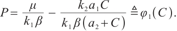
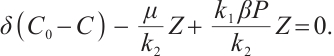
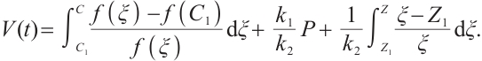
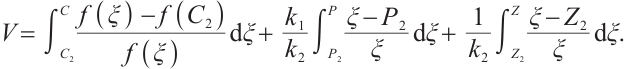
To investigate the coexistence equilibrium, we first substitute the zooplankton density from (7) into the carbon balance equation (8), a key step in linking phytoplankton and TOC dynamics. Subsequently, by performing algebraic manipulation (i.e., multiplying both sides by  ), we obtain the following algebraic equation:
 (10)
(10)
This equation describes the balance between TOC input and planktonic nutrient cycling. Solving equation (10) leads to the expression
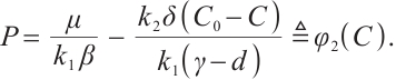 (11)
(11)
From (6) it is easy to see that 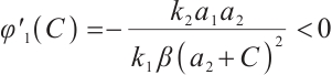 . Thus,
  is a strictly decreasing and continuous function of
  . It should also be noted that
 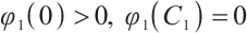 , and
, and 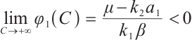 if
if  .
.
Similarly, from (11) we know that 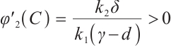 . Given that
  this derivative indicates that
 is a strictly increasing and continuous function of
  . It is straightforward to see that
Let  . Then
  if
if  , and
, and  .
.
Thus, the equation  admits a unique positive solution if and only if
  , i.e.,
  . Consequently, the unique coexistence equilibrium
  exists when
  . This equilibrium includes TOC, phytoplankton, and zooplankton, with
  ,
,  , and
, and  being the solution to the equation
The previous analysis can be summarized as follows.
Theorem 2 For system (1), the plankton-free equilibrium  always exists. When
  , the phytoplankton-free equilibrium
  exists for
  , where
  Meanwhile, the unique coexistence equilibrium
  exists if and only if
  , where
  is the unique solution to
  , and
, and  .
.
2 Stability of Equilibria
In this section, we will discuss the asymptotic stability of equilibria  ,
,  , and
, and  for system (1).
First, we investigate the local stability of equilibrium points, with a primary emphasis on the eigenvalues of the Jacobian matrices calculated at each specific equilibrium. Formally, an equilibrium point is locally asymptotically stable if every eigenvalue of its Jacobian matrix has a negative real part. In particular, the real eigenvalues must be strictly negative, and complex eigenvalues must have negative real parts.
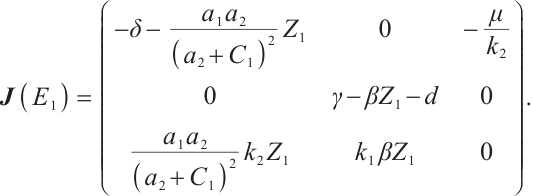
The Jacobian matrix  of system (1) at any point
  in the positive quadrant
  is given by
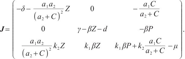 (12)
(12)
The subsequent theorem characterizes the local asymptotic stability of equilibria for system (1).
Theorem 3 The plankton-free equilibrium  is unstable because the Jacobian matrix
  has at least one eigenvalue with a positive real part
 The phytoplankton-free equilibrium
  is locally asymptotically stable if and only if
  . Conversely, the unique coexistence equilibrium
  is locally asymptotically stable when
  .
.
Proof The Jacobian matrix for system (1) at the plankton-free equilibrium  is determined by
 (13)
(13)
The characteristic equation corresponding to  is derived as
 (14)
(14)
Solving (14), the eigenvalues are obtained as  ,
,  ,
,  .
. Since
Since  , it follows that
 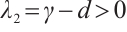 .
.
The plankton-free equilibrium  is unstable because the eigenvalue
  is positive.
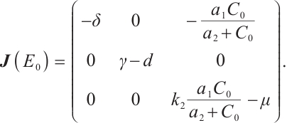
When phytoplankton-free equilibrium  exists, its Jacobian matrix is
 (15)
(15)
One of the eigenvalues of (15) is 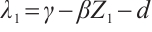 . Substituting
 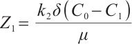 and
and 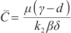 into this expression, we have
  .
.
It follows that
 (16)
(16)
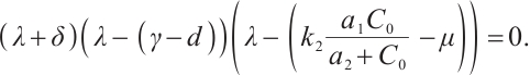
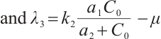
The other eigenvalues  and
and  are determined by the equation
where 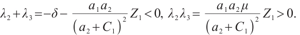 Thus,
Thus, 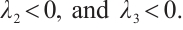
Consequently, all eigenvalues of the Jacobian matrix (15) exhibit negative real parts under the condition  . Therefore, the phytoplankton-free equilibrium
  is locally asymptotically stable when it satisfies
  .
.
When coexistent equilibrium  exists, the Jacobian matrix at
  is
is
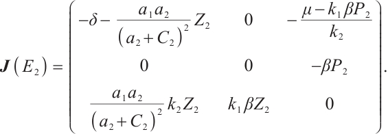 (17)
(17)
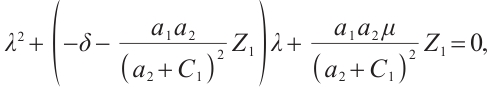
The characteristic equation for the coexistence equilibrium  can be written as
 (18)
(18)
where  , and
, and  .
.
From equation (6), we readily deduce that 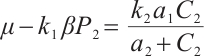 . Substituting this expression into
  , we rewrite it as
 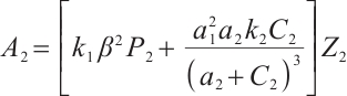 . As stated in Theorem 2, when
  , system (1) has a unique positive equilibrium
  , with
  . All terms within the expression for
  are positive when
  . This directly verifies that
  when the coexistence equilibrium exists.
These results indicate that

By the Routh-Hurwitz stability criterion[25], it follows that all eigenvalues of equation (18) have negative real parts. Consequently, the unique coexistence equilibrium  is locally asymptotically stable if and only if
  . This completes the proof of Theorem 3.
Next, we will establish the global stability of the equilibria  and
and  using the Lyapunov-LaSalle theorem[26].
Theorem 4 The phytoplankton-free equilibrium  is globally asymptotically stable if and only if
  .
.
Proof Let  . Define a Lyapunov function as
 (19)
(19)
Along the trajectories of system (1), computing the time derivative of  yields
 (20)
(20)
Substituting  and
and  into (20), we obtain
 (21)
(21)
It follows from equation (16) that  when
when  . Note that
  is a positive increasing function, and solutions of system (1) remain nonnegative. Thus, all terms in (21) are non-positive, implying
  . Furthermore
  if and only if
  ,
,  , and
, and  . Therefore,
  is the largest invariant subset of system (1). By Lyapunov-LaSalle invariant principle and Theorem 3[26],
  is globally asymptotically stable when
  . This completes the proof.
Theorem 5 The unique coexistence equilibrium  is globally asymptotically stable if and only if
  .
.
Proof We make the same assumption  , and define a new Lyapunov function
 (22)
(22)
By calculating the time derivative of  along the trajectories of system (1), we obtain
 (23)
(23)
Following a similar approach to analyze the global asymptotic stability of  , substituting
  and
and  into the Lyapunov function yields
 (24)
(24)
Clearly,  holds when
  , i.e.,
  . Furthermore,
  if and only if
  ,
,  , and
, and  .
.
Thus, any solution of system (1) tends to  , which is the maximal invariant subset of system (1). By applying the Lyapunov⁃LaSalle theorem in conjunction with Theorem 3, the global asymptotic stability of
  is established. The proof is completed.
3 Simulation Results
In this section, we use numerical simulations to investigate the global dynamics of model (1) for the input concentration threshold value  .
.
The values of these parameters are set as follows.

From the specified parameter values, it is evident that  ,
,  , which satisfy the condition
  in Theorem 5. The globally asymptotically stable coexistence equilibrium
  implies that phytoplankton and zooplankton populations will converge to a stable coexistence state under low TOC inputs. This theoretical prediction is validated by the numerical simulation results shown in Fig. 1. Figure 1(a) illustrates that TOC-phytoplankton-zooplankton dynamics exhibit limit cycle behavior. Figure 1(b) reveals that the amplitude of phytoplankton density trajectories surpasses that of TOC concentration trajectories, thereby indicating that the fluctuations in phytoplankton density are more pronounced than those in TOC concentration. Figure 1 suggests that phytoplankton play a critical role in promoting zooplankton growth and highlights zooplankton’s feeding preference for phytoplankton. By contrast, even minor TOC additions dampen oscillation amplitudes, leading to asymptotic stabilization of phytoplankton density. This suggests that lentic ecosystems are highly susceptible to trophic destabilization from low-level allochthonous subsidies.
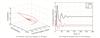 |
Fig. 1 Stable behavior of  for for 
|
The influx of allochthonous organic matter varies among lakes. Therefore, we explore the impact of threshold  variations on ecosystem dynamics in Fig. 2. Increasing
  to 15 while maintaining other parameters constant, we obtain
  , and
, and 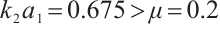 . According to Theorem 4, the equilibrium
 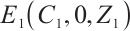 is globally asymptotically stable under sufficiently high input TOC concentration.
 |
Fig. 2 Stable behavior of  for for 
|
When the concentration of the input TOC is increased to  , Fig. 2(a) confirms that
  is asymptotically stable. As depicted in Fig. 2(b), the amplitude of allochthonous organic matter concentration trajectories exceeds that of phytoplankton density trajectories. These results imply that fluctuations in allochthonous organic matter are more pronounced than those in phytoplankton. Simulation in Fig. 2 demonstrates that phytoplankton density declines to zero, signifying the extinction of this population. At the point
  , when
  , the condition
  holds. This imbalance results in a negative net growth rate for phytoplankton, hence insufficient to sustain positive population growth. The predation pressure
  exceeding the phytoplankton survival threshold triggers the extinction cascade. Moreover, Fig. 2 shows a corresponding increase in zooplankton density concurrent with phytoplankton decline, implying that zooplankton growth is influenced by allochthonous organic matter, TOC exerts inhibitory effects on phytoplankton through the term
  . Specifically, zooplankton exhibits a preference for external resources. A high allochthonous organic carbon influx may suppress phytoplankton growth, potentially causing extinction. This results from zooplankton consuming terrestrial organic carbon, which indirectly inhibits phytoplankton via trophic cascades. TOC boosts zooplankton biomass, thereby increasing predation pressure on phytoplankton through higher grazing rates. This paper emphasizes an important conclusion that the input TOC concentration influences equilibrium states and stability.
4 Conclusion
In order to explore the ecological role of TOC in lake ecosystems, a novel terrestrial organic carbon-phytoplankton-zooplankton model is proposed, where zooplankton consumption of TOC follows a Holling type Ⅱ functional response. Theoretical analysis and numerical simulations reveal that the input TOC concentration  is a key factor which influences the dynamics of model (1).
Theorem 4 formalizes that zooplankton can persist indefinitely even in the absence of phytoplankton, provided TOC influx exceeds a critical threshold, especially in nutrient-poor lakes. Moreover, fluctuations in TOC input concentrations have been demonstrated to govern the observed ecological dynamics. Specifically, results derived from system (1) provide robust corroboration for the hypotheses postulated in Ref. [24]. This work extends the classic phytoplankton-zooplankton modeling paradigm by demonstrating that TOC not only serves as an alternative carbon source but also restructures trophic interactions.
Notably, the model underscores the importance of terrestrial-aquatic carbon coupling for maintaining ecosystem resilience. Mechanistically, increased TOC inputs may inhibit phytoplankton blooms via resource dilution, leading to stable zooplankton densities. These findings advocate for regulating TOC input as a viable management approach to control harmful algal blooms, particularly in bloom-prone lakes.
The paper’s primary shortcoming resides in the model’s restricted validation scope, which is confined to scenarios with low filter-feeder biomass (e.g., early-stage eutrophication). New modules are imperative for high-predation environments such as shellfish farms. For intensive predation scenarios (e.g., commercial shellfish aquaculture), the future research will implement ecological complexity integration via modular design. The proposed extension involves incorporating filter-feeder functional groups (e.g., fish), thereby expanding the system into a four-variable dynamic framework.
References
- Fry B. Stable Isotope Ecology[M]. New York: Springer-Verlag, 2006. [Google Scholar]
- Richardson J S, Zhang Y X, Marczak L B. Resource subsidies across the land-freshwater interface and responses in recipient communities[J]. River Research and Applications, 2010, 26(1): 55-66. [Google Scholar]
- Sleighter R L, Hatcher P G. The application of electrospray ionization coupled to ultrahigh resolution mass spectrometry for the molecular characterization of natural organic matter[J]. Journal of Mass Spectrometry, 2007, 42(5): 559-574. [Google Scholar]
- Cole J J, Carpenter S R, Pace M L, et al. Differential support of lake food webs by three types of terrestrial organic carbon[J]. Ecology Letters, 2006, 9(5): 558-568. [Google Scholar]
- Wetzel R G. Limnology: Lake and River Ecosystems[M]. London: Elsevier Academic Press, 2001. [Google Scholar]
- Pace M L, Cole J J, Carpenter S R, et al. Whole-lake carbon-13 additions reveal terrestrial support of aquatic food webs[J]. Nature, 2004, 427(6971): 240-243. [Google Scholar]
-
Carpenter S R, Cole J J, Pace M L, et al. Ecosystem subsidies: Terrestrial support of aquatic food webs from
 addition to contrasting lakes[J]. Ecology, 2005, 86(10): 2737-2750.
[Google Scholar]
addition to contrasting lakes[J]. Ecology, 2005, 86(10): 2737-2750.
[Google Scholar]
- Solomon C T, Carpenter S R, Clayton M K, et al. Terrestrial, benthic, and pelagic resource use in lakes: Results from a three-isotope Bayesian mixing model[J]. Ecology, 2011, 92(5): 1115-1125. [Google Scholar]
- Pace M L, Carpenter S R, Cole J J, et al. Does terrestrial organic carbon subsidize the planktonic food web in a clear-water lake?[J]. Limnology and Oceanography, 2007, 52(5): 2177-2189. [Google Scholar]
- Yokokawa T, Nagata T. Linking bacterial community structure to carbon fluxes in marine environments[J]. Journal of Oceanography, 2010, 66(1): 1-12. [Google Scholar]
- Boschker H T S, Middelburg J J. Stable isotopes and biomarkers in microbial ecology[J]. FEMS Microbiology Ecology, 2002, 40(2): 85-95. [Google Scholar]
- Berggren M, Ström L, Laudon H, et al. Lake secondary production fueled by rapid transfer of low molecular weight organic carbon from terrestrial sources to aquatic consumers[J]. Ecology Letters, 2010, 13(7): 870-880. [Google Scholar]
- Speas D W, Duffy W G. Uptake of dissolved organic carbon (DOC) by daphnia pulex[J]. Journal of Freshwater Ecology, 1998, 13(4): 457-463. [Google Scholar]
- Pei Y Z, Lv Y F, Li C G. Evolutionary consequences of harvesting for a two-zooplankton one-phytoplankton system[J]. Applied Mathematical Modelling, 2012, 36(4): 1752-1765. [Google Scholar]
- Li Y F, Liu H C, Yang R Z, et al. Dynamics in a diffusive phytoplankton-zooplankton system with time delay and harvesting[J]. Advances in Difference Equations, 2019, 2019(1): 79. [Google Scholar]
- Saha T, Bandyopadhyay M. Dynamical analysis of toxin producing phytoplankton-zooplankton interactions[J]. Nonlinear Analysis: Real World Applications, 2009, 10(1): 314-332. [Google Scholar]
- Chakraborty K, Das K. Modeling and analysis of a two-zooplankton one-phytoplankton system in the presence of toxicity[J]. Applied Mathematical Modelling, 2015, 39(3/4): 1241-1265. [Google Scholar]
- Lv Y F, Cao J Z, Song J, et al. Global stability and Hopf-bifurcation in a zooplankton-phytoplankton model[J]. Nonlinear Dynamics, 2014, 76(1): 345-366. [Google Scholar]
- Rehim M, Imran M. Dynamical analysis of a delay model of phytoplankton-zooplankton interaction[J]. Applied Mathematical Modelling, 2012, 36(2): 638-647. [Google Scholar]
- Ruan S G. The effect of delays on stability and persistence in plankton models[J]. Nonlinear Analysis: Theory, Methods & Applications, 1995, 24(4): 575-585. [Google Scholar]
- Fan A J, Han P, Wang K F. Global dynamics of a nutrient-plankton system in the water ecosystem[J]. Applied Mathematics and Computation, 2013, 219(15): 8269-8276. [Google Scholar]
- Zhang T R, Wang W D. Hopf bifurcation and bistability of a nutrient-phytoplankton-zooplankton model[J]. Applied Mathematical Modelling, 2012, 36(12): 6225-6235. [Google Scholar]
- Tanentzap A J, Kielstra B W, Wilkinson G M, et al. Terrestrial support of lake food webs: Synthesis reveals controls over cross-ecosystem resource use[J]. Science Advances, 2017, 3(3): e1601765. [Google Scholar]
- Brett M T, Kainz M J, Taipale S J, et al. Phytoplankton, not allochthonous carbon, sustains herbivorous zooplankton production[J]. Proceedings of the National Academy of Sciences of the United States of America, 2009, 106(50): 21197-21201. [Google Scholar]
- Routh E J. A Treatise on the Stability of a Given State of Motion[M]. London: Macmillan Publishers, 1877. [Google Scholar]
- La Salle J P. The extent of asymptotic stability[J]. Proceedings of the National Academy of Sciences of the United States of America, 1960, 46(3): 363-365. [Google Scholar]
All Figures
|
Fig. 1 Stable behavior of for
|
| In the text | |
|
Fig. 2 Stable behavior of for
|
| In the text | |
Current usage metrics show cumulative count of Article Views (full-text article views including HTML views, PDF and ePub downloads, according to the available data) and Abstracts Views on Vision4Press platform.
Data correspond to usage on the plateform after 2015. The current usage metrics is available 48-96 hours after online publication and is updated daily on week days.
Initial download of the metrics may take a while.