| Issue |
Wuhan Univ. J. Nat. Sci.
Volume 30, Number 3, June 2025
|
|
|---|---|---|
| Page(s) | 213 - 221 | |
| DOI | https://doi.org/10.1051/wujns/2025303213 | |
| Published online | 16 July 2025 | |
Computer Science
CLC number: TP399
Study on the Effect of Spot Size and Non-Linearity on PSD Positioning Accuracy
光斑尺寸及非线性度对PSD定位精度影响研究
1 School of Electronic and Electrical Engineering, Shanghai University of Engineering Science, Shanghai 201620, China
2 School of Optical-Electrical and Computer Engineering, University of Shanghai for Science and Technology, Shanghai 200093, China
† Corresponding author. E-mail: This email address is being protected from spambots. You need JavaScript enabled to view it.
Received:
2
December
2024
Abstract
Position-sensitive detector (PSD) is widely used in precision measurement fields such as flatness detection, auto-collimator systems, and degrees of freedom testing. However, due to factors such as uneven surface resistance and differences in electrode structures, the nonlinearity of PSD becomes increasingly severe as the photosensitive surface moves from the center toward the edges of the four electrodes. To address this issue, a PSD nonlinearity correction algorithm is proposed. The algorithm utilizes the particle swarm optimization (PSO) algorithm to determine the optimal weights and thresholds, providing better initial parameters for the back propagation (BP) neural network. The BP neural network then iterates continuously until the error conditions are met, completing the correction process. Furthermore, a PSD nonlinearity correction system was developed, and the influence of different spot sizes on PSD positioning accuracy was simulated based on the current equation under the Gaussian spot model. This validated the robustness of the correction algorithm under varying spot sizes. The results demonstrate that the overall optimized error is reduced by 84.51%, and for spot sizes smaller than 1 mm, the error reduction exceeds 93.89%. This method not only meets the measurement accuracy requirements but also extends the measurement range of PSD.
摘要
位置敏感探测器(PSD)被广泛应用于平整度检测、自准直仪系统及自由度测试等精密测量领域。然而,由于表面电阻不均匀和电极结构差异等因素,PSD的非线性问题在光敏表面从中心向四个电极的边缘靠近时变得越来越严重。针对这一问题,提出了一种PSD非线性校正算法,利用粒子群(PSO)算法计算出最佳权值和阈值,为BP神经网络提供较好的初始参数,再通过BP神经网络不断迭代,直到满足误差条件,完成校正过程。此外,构建了PSD非线性校正系统,根据高斯光斑模型条件下的电流方程,仿真不同的光斑尺寸对PSD定位精度的影响,验证了校正算法在不同光斑尺寸下的鲁棒性。结果表明,优化后的整体误差减少了84.51%,当光斑尺寸小于1mm时,误差减少超过93.89%。该方法不仅满足了测量精度要求,还扩展了PSD的测量范围。
Key words: position-sensitive detector / particle swarm algorithm / nonlinear optimization / spot characteristics / positioning accuracy
关键字 : 位置敏感探测器 / 粒子群算法 / 非线性优化 / 光斑特性 / 定位精度
Cite this article: WANG Zechuan, ZHANG Zhenhua, CHENG Shaowei, et al. Study on the Effect of Spot Size and Non-Linearity on PSD Positioning Accuracy[J]. Wuhan Univ J of Nat Sci, 2025, 30(3): 213-221.
Biography: WANG Zechuan, male, Master candidate, research direction: 3D measurement. E-mail: This email address is being protected from spambots. You need JavaScript enabled to view it.
Foundation item: Supported by the National Natural Science Foundation of China (U1831133); Open Fund of Key Laboratory of Space Active Optoelectronics Technology, Chinese Academy of Sciences (2021ZDKF4)
© Wuhan University 2025
 This is an Open Access article distributed under the terms of the Creative Commons Attribution License (https://creativecommons.org/licenses/by/4.0), which permits unrestricted use, distribution, and reproduction in any medium, provided the original work is properly cited.
0 Introduction
Position-sensitive detectors (PSDs) are current-distributing photoelectric devices with a continuous photosensitive surface, capable of rapidly responding to the centroid position of a light spot irradiated on their surface. Due to their high positional resolution, simple signal processing, and excellent measurement continuity, PSDs are widely applied in scenarios with stringent real-time requirements, such as flatness detection[1], real-time coaxiality measurement[2], and robotic arm trajectory monitoring[3].
In 1960, Lucovsky et al [4] derived a differential equation describing the photoelectric potential distribution of a two-dimensional planar P-N junction based on the continuity equation of carriers, thereby establishing the theoretical foundation for PSD modeling. Despite their advantages of fast response speed and high resolution, PSDs are significantly affected by the non-uniformity of surface resistance and substantial interference between electrodes, which severely degrade the detector's linearity. Since PSDs measure the intensity of incident light spots, the size of the laser spot and the effectiveness of subsequent nonlinear optimization directly determine measurement accuracy. Wang et al[5] proposed a neural network-based correction approach for PSD, establishing a mapping between actual output and spot position with a limited dataset, which resulted in highly linear signals over a wide range. Shang et al[6] investigated various light source scanning methods and concluded that the scanning method under steady-state illumination more accurately reflects the position information of the incident light. Li et al[7] analyzed the impact of light source modes on PSD positioning accuracy, identifying spot radius and position as the primary influencing factors. Huang et al [8] demonstrated that processing PSD output signals under strong background light interference can effectively improve the spatial accuracy of flashpoint position measurements. Zhang et al [9] developed a PSD nonlinear correction method based on the BP optimization algorithm, demonstrating strong generalization ability and feasibility in resolving PSD nonlinearity by fitting actual and ideal position data using a BP neural network. Wang et al[10] corrected the nonlinear distortion of PSD using an improved bicubic interpolation method, achieving favorable results even under dynamic spot conditions.
Building upon this prior research, this paper derives a two-dimensional PSD positioning model under varying spot sizes within a Gaussian spot framework, based on the mathematical model of the Lucovsky differential equation. A nonlinear optimization method combining the Particle Swarm Optimization (PSO) algorithm and the BP neural network is proposed. By correcting measurement errors based on the relationship between input and output values, the proposed method yields predicted values that approximate the true coordinates. Additionally, the effects of different spot sizes on positioning accuracy are analyzed, providing practical insights for improving PSD measurement accuracy.
1 Principle of PSD
A position-sensitive detector (PSD) is a spot position detector based on the semiconductor lateral photoelectric effect. Its structure consists of a P-I-N junction formed by P-type, N-type semiconductors, along with a high-resistance I layer[11]. Figure 1 shows the basic structure of a pillow-shaped two-dimensional PSD, which is an improved version of a quadrilateral PSD. The top surface of the pillow-shaped PSD is a photosensitive surface with arc-shaped electrodes, while the four sides are connected to four current output terminals symmetrically drawn from the arc-shaped edges. The bottom surface has a common cathode. The four current output terminals, X1 , X2 , Y1 , and Y2 , collect different currents generated by the distances between the spot centroid incident on the photosensitive surface and the respective electrodes. By calculating these currents, the position coordinates of the spot can be determined. The common cathode is used to apply a reverse bias voltage during operation to achieve ideal linearity.
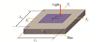 |
Fig. 1 Pincushion-type PSD structure model |
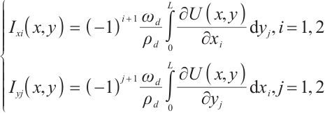
When incident light projects onto the photosensitive surface of the PSD, forming a light spot, the lateral photoelectric effect converts the incident light into photocurrent. The output current intensities at the four electrode terminals correspond to the x and y coordinates of the spot centroid. Using the following equations, the coordinate equations with the photosensitive surface center as the origin[12] can be calculated:
 (1)
(1)
where  ,
, ,
, ,
, are the voltage values obtained by the four current output electrodes after converting the voltage signals by photocurrent and amplifying them,
  and
and  are the two side lengths of the 2D PSD photosensitive surface, respectively, and
  is usually used.
2 Nonlinear Optimization of PSD
2.1 Causes of Nonlinearity
The structure of the pillow-shaped two-dimensional PSD consists of a single-sided resistive layer for current distribution. In equation (1), the electrode junctions of the pillow-shaped two-dimensional PSD are considered idealized in terms of shape and size. However, due to manufacturing process limitations, the PN junction material of the PSD cannot ensure a uniform distribution of the resistive layer. As a result, the output electrodes often exhibit variations in size and shape, leading to a nonlinear relationship between the detected light spot position coordinates and the actual PSD output during measurement. This nonlinearity increases with the distance from the center of the photosensitive surface. Consequently, the photosensitive surface of the PSD is typically divided into two regions: Zone A and Zone B. Zone A is defined as the area within a diameter that is 40% of the boundary length of the photosensitive surface centered on its center, while Zone B covers the region between 40% and 80% of the boundary length. The positional accuracy in Zone A is superior to that in Zone B. Therefore, when it is necessary to use the entire photosensitive surface to expand the measurement range without compromising accuracy, it is essential to correct for the nonlinearity of the PSD.
2.2 PSO-BP Neural Network
A BP (back propagation) neural network is a multilayer feedforward neural network that uses error backpropagation. The structure of the neural network includes an input layer, hidden layers, and an output layer. The relationship between the output and input can be seen as a mapping. This mapping is obtained through the transfer functions between the input layer and the hidden layer, the hidden layers and the hidden layers, and the hidden layer and the output layer[13]. The BP neural network, with its robust nonlinear modeling capability, self-learning and adaptive characteristics, strong generalization ability, and proficiency in handling multivariable inputs, serves as an optimal choice for addressing the nonlinear challenges in PSD analysis.
Due to the BP neural network's excessive reliance on the initial weights and thresholds, it often suffers from poor generalization ability and is prone to getting stuck in local optima. To enhance the effectiveness of the algorithm, a particle swarm optimization (PSO) algorithm is introduced. The PSO algorithm, proposed by Kennedy and Eberhart, is a parallel optimization algorithm inspired by the collective behavior of bird flocks and fish schools in nature[14]. It is a powerful global optimization algorithm with advantages such as strong global search capability, no need for gradient information, the ability to perform multi-objective optimization, and the ability to balance global and local optima. Similar to the genetic algorithm (GA), PSO incorporates the concept of interacting populations. In many applications, PSO has been demonstrated to converge more rapidly to the optimal solution compared with GA[15].The PSO has N individual particles combining self-experience and social experience, and the corresponding position of each particle is a solution. The first  particle
  starts "flying" in the M-dimensional search space at a random position with a certain speed, and its position and speed are expressed as
  and
and  , which moves towards the optimal solution in the search space, and finally reaches the global optimum. The positions and velocities are updated from generation
  to generation
  as follows:
 (2)
(2)
where  is the inertia weights to regulate the global search,
  and
and  are the individual learning coefficients and the sociological coefficients respectively,
  and
and  are the random numbers within the range of
  in the iterative process, and
  and
and  generate the individual optimal solution and the global optimal solution through each update.
However, the standard PSO algorithm tends to exhibit rapid population convergence due to large inertia in the early stages, making it prone to getting trapped in local optima. To balance global and local search capabilities, dynamically adjusted inertia weights  are used during the search process. Shi et al[16] proposed a linearly decreasing inertia factor:
 (3)
(3)
where  and
and  are the initial and final values of the inertia factor,
  is the current number of iterations, and
  is the final number of iterations.
Compared with the BP neural network, the PSO algorithm exhibits superior global search capabilities. The process of using PSO to optimize the BP neural network is shown in Fig. 2.
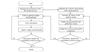 |
Fig. 2 Flow chart of PSO-BP model |
The specific steps are as follows:
1) Initialize the parameters of the BP neural network, including setting the weights and thresholds.
2) Initialize the parameters of the PSO, including setting the population size, initial velocity, and position of the particles.
3) Calculate the fitness of the particles, generating individual best and global best values.
4) Update the velocity and position of the particles based on the individual best and global best values. If the stopping criterion is met, proceed to step 5); otherwise, return to step 3) and repeat.
5) Use the optimized weights and thresholds obtained from the PSO to initialize the BP neural network.
6) Compute the error through the neural network and continuously update the weights and thresholds.
7) Check if the error meets the specified requirements. If not, return to step 6) and continue until the stopping criterion is met, then terminate the training.
3 The Effect of Spot Size on PSD Accuracy
Since the PSD photosensitive surface receives the coordinates of the incident light spot's center of gravity, and the size of the photosensitive surface is limited, the nonlinearity increases as it approaches the edges of the photosensitive surface[17]. Therefore, it is essential to study the impact of different sizes of incident light spots on positioning accuracy. According to the Lucovsky differential equation, under the ideal condition where the spot energy is converted to photocurrent without loss, the potential at the point  on the photosensitive surface can be expressed as:
 (4)
(4)
where  represents the potential at the light spot detected on the photosensitive surface,
  denotes the Laplace operator,
  is the resistivity of the P layer,
  is the thickness of the P layer,
  is the total photocurrent at the light spot
  , and the currents at the four electrodes of the PSD can be calculated by the following equations:
 (5)
(5)
where  and
and  are the electrode currents,
  is the length of the edge electrodes on the PSD's photosensitive surface. Assuming the boundary length of the PSD is one standard unit and taking the center of the PSD's photosensitive surface as the coordinate origin, the junction potential equation can be derived from partial differential equation (4) under the condition of zero electrode potential:
 (6)
(6)
where  is the effective area of the 2D PSD photosensitive surface, and the polar coordinate transformation of (6) is performed:
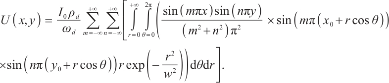 (7)
(7)
Available after integrating  :
:
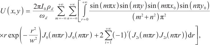 (8)
(8)
where  denotes the Bessel function and the Bessel function formula is as follows:
 (9)
(9)
 (10)
(10)
where  denotes the modified Type I Bessel function, and the potential is calculated by solving the integral over
  :
:
 (11)
(11)
From this, the current equations for the four electrodes can be calculated:
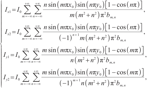 (12)
(12)
To analyze the impact of different spot sizes on the photosensitive surface on the positioning accuracy, a simulation experiment was designed to simulate the calculation of position coordinates under varying spot sizes. The photocurrent  was set to one unit, and the length of the photosensitive surface
  was assumed to be nine units. The spot moved across the PSD photosensitive surface with a step size of 0.5 units, simulating four different spot sizes:
  ,
,  ,
,  , and
, and  , generating a
  grid of discretized data points, totaling 289 position coordinates. The distribution of the simulated position coordinates for the different spot sizes is shown in Fig. 3.
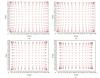 |
Fig. 3 Simulation of position coordinates calculation for different spot sizes (a) at |


As shown in the figure, within the Zone A of the photosensitive surface, different spot sizes exhibit good linearity. However, in the Zone B, significant non-linear phenomena are observed due to edge current effects. Additionally, as the spot size increases, the positioning accuracy of the PSD photosensitive surface significantly decreases.
4 Experiment
4.1 Experimental Platform
In order to investigate the impact of different spot sizes and non-linearity on positioning accuracy, a nonlinear optimization experimental platform was established, as shown in Fig. 4. The effective length of the PSD photosensitive surface is  , which is fixed on a precision displacement platform. A semiconductor laser is mounted on a three-dimensional moving platform, with adjustable spot size. By controlling the three-dimensional moving platform to scan the entire photosensitive surface of the PSD with a step size of 1 mm, a total of 100 discrete coordinate data points at
  different positions were obtained. To ensure measurement accuracy, the entire experiment was conducted under dark background conditions.
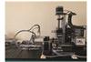 |
Fig. 4 Nonlinear optimization experimental platform |
4.2 Algorithm Robustness
Figure 5 compares the measured coordinate data and the positions after nonlinear optimization. As seen in the figure, the actual measured positions show a pincushion distortion compared with the standardized grid. Within Zone A, the linearity is relatively good; however, as the distance from the central point increases, significant nonlinear distortion occurs in Zone B, with the distortion being more pronounced at the four electrode ends at the outermost edges. Therefore, to extend the effective usage area of the PSD photosensitive surface while maintaining accuracy, it is necessary to correct for nonlinear errors. After applying the PSO-BP correction, the linearity of the corrected positions shows a significant improvement compared with the measured positions. The comparison with the standard position coordinates visually demonstrates that the nonlinear distortion is largely eliminated.
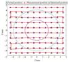 |
Fig. 5 Comparison of position coordinates before and after nonlinear optimization |
By adjusting the laser spot diameter projected onto the photosensitive surface and collecting the measurement coordinates for different spot diameters, the comparison between the actual position coordinates and the optimized coordinates is shown in Fig. 6.
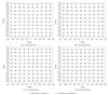 |
Fig. 6 Measured and optimized values for different light spots |
In Fig.6, (a) , (b) , (c) , and (d) show the comparison result between the measured coordinates and the optimized coordinates for laser spots with diameters of 0.5 mm, 1.0 mm, 1.5 mm, and 2.0 mm, respectively. It can be observed that as the spot diameter increases, the accuracy of the PSD in detecting the laser spot position decreases, and the degree of nonlinear distortion increases. However, after optimization with the PSO-BP algorithm, the linearity significantly improves.
4.3 Error Analysis
Due to the varying degrees of distortion in the Zones A and B of the photosensitive surface, the significance of nonlinear optimization is also affected. To clearly distinguish the optimization significance between the Zones A and B, we selected and compared the position coordinates of the same light spot along the same diagonal under four different spot sizes.
After nonlinear optimization of the position coordinates obtained from laser spots of various sizes on the PSD's photosensitive surface, the error can be used to evaluate the effectiveness of linearity optimization. The optimization results for Zone A of the photosensitive surface are shown in Fig. 7. In Zone A, within 40% of the distance from the center of the photosensitive surface, linearity remains good. Under the condition of a spot size of  , the average error after optimization in Zone A is controlled to within
  , achieving an optimization level of 95.19% compared with the pre-optimization error. As the spot size increases, the level of optimization gradually decreases, with errors reducing by more than 85.39% when the spot size reaches
  .
.
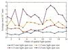 |
Fig. 7 Comparison of the average error of Zone A under different spot sizes |
Figure 8 shows the optimization results for Zone B of the photosensitive surface. The figure indicates that when the spot size is below  , the results of nonlinear optimization are significant, with the average error after optimization reduced by more than 93.89%. However, when the spot size reaches
  , the optimization effect shows a significant weakening trend, and the average error reduced by 72.58%. This indicates that smaller spot diameters result in more concentrated energy, leading to higher positioning accuracy for the PSD. Considering the nonlinear optimization results for various spot sizes across both Zone A and Zone B of the photosensitive surface, the average positioning error was reduced by 84.51% after optimization.
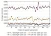 |
Fig. 8 Comparison of the average error of Zone B under different spot sizes |
5 Conclusion
In this paper, we derived the Lucovsky differential equation mathematical model for the PSD and obtained a positioning model for the two-dimensional PSD under different spot sizes. Through simulation, we found that as the spot size increases, the positioning accuracy decreases. To address the inherent nonlinear distortion issues of the PSD, we employed a particle swarm optimization algorithm to improve the BP neural network nonlinear optimization method. The optimization significantly reduced the nonlinear errors in both the Zone A and B, effectively eliminating the pillow-shaped distortion. Moreover, the nonlinear distortion of different spot sizes projected onto the photosensitive surface was reliably corrected, with an average optimization improvement of over 84.51%, especially achieving over 93.89% for spots smaller than  . This greatly reduced the positioning error of the detector. Based on the research presented, the effective usable area of the photosensitive surface can be increased, and the positioning accuracy of the PSD can be enhanced, enabling the two-dimensional PSD to be applied in wide-range and high-precision measurement systems.
References
- Han J Y, Wang S Z. Research on the method of applying position sensitive detector to detect flatness[J]. Combined Machine Tools and Automated Machining Technology, 2016(7): 82-85(Ch). [Google Scholar]
- Quan L Y, Tan J P, Wang X, et al. Research on real-time inspection system for high precision extrusion machine centerline coaxiality[J]. Forging and Pressing Technology, 2012, 37(3): 73-77(Ch). [Google Scholar]
- Lu X H, Wang W T, Si L K, et al. Dual PSD-based robotic motion trajectory tracking measurement device[J]. Manufacturing Technology and Machine Tools, 2015(6): 61-66(Ch). [Google Scholar]
- Lucovsky G. Photoeffects in nonuniformly irradiated P-N junctions[J]. Journal of Applied Physics, 1960, 31(6): 1088-1095. [Google Scholar]
- Wang X D, Ye M Y. Nonlinear correction of two-dimensional optoelectronic position-sensitive devices[J]. Optical Technology, 2002(2): 174-175+178. [Google Scholar]
- Shang H Y, Zhang G J. Response characteristics of PSD based on two scanning methods[J]. Journal of Instrumentation, 2005(11): 34-38(Ch). [Google Scholar]
- Li K, Xuan R X, Zhang H M, et al. Influence of light source on the positioning accuracy of position-sensitive sensors[J]. Journal of Hubei Automotive Industry College, 2010, 24(2): 37-40(Ch). [Google Scholar]
- Huang Z H, Li X D, Cai H Y, et al. Research on PSD-based optical spot position detection technology in strong background[J]. Optical Engineering, 2012, 39(10): 89-94(Ch). [Google Scholar]
- Zhang X T, Kang L, Wu Q Q, et al. Nonlinear correction of PSD based on BP optimization algorithm[J]. Journal of Applied Optics, 2016, 37(3): 415-418(Ch). [Google Scholar]
- Wang J Y, Wang X D, Liu Z, et al. Nonlinear distortion correction algorithm for two-dimensional PSD[J]. Journal of Wuhan University of Science and Technology, 2019, 42(1): 56-60(Ch). [Google Scholar]
- Teng Y K, Hao Y M, Fu S F, et al. Calibration technique for position-sensitive device based visual measurement system[J]. Advances in Laser and Optoelectronics, 2018, 55(8): 304-311. [Google Scholar]
- Zhang P C, Liu J, Yang H M, et al. Research on non-uniform laser spot center localization based on PSD[J]. Laser and Infrared, 2020, 50(8): 941-947(Ch). [Google Scholar]
- Liu X, Liu Z, Liang Z, et al. PSO-BP neural network-based strain prediction of wind turbine blades[J]. Materials (Basel), 2019, 12(12): 1889. [Google Scholar]
- Yu J Q, Gao Z K, Zhao A J, et al. Improved parallel particle swarm algorithm for energy saving optimization of cooling water systems[J]. Control Theory and Applications, 2022, 39(3): 11(Ch). [Google Scholar]
- Banks A, Vincent J, Anyakoha C. A review of particle swarm optimization. Part I: Background and development[J]. Natural Computing, 2007, 6(4): 467-484. [Google Scholar]
- Shi Y, Eberhart R. A modified particle swarm optimizer[C]// 1998 IEEE International Conference on Evolutionary Computation Proceedings. IEEE World Congress on Computational Intelligence. New York: IEEE, 1998: 69-73. [Google Scholar]
- Meng N, Zeng J R, Li Z L, et al. Position detection of synchrotron light spot based on position-sensitive semiconductor optoelectronic devices[J]. Nuclear Technology, 2020, 43(12): 18-26(Ch). [Google Scholar]
All Figures
|
Fig. 1 Pincushion-type PSD structure model |
| In the text | |
|
Fig. 2 Flow chart of PSO-BP model |
| In the text | |
|
Fig. 3 Simulation of position coordinates calculation for different spot sizes (a) at |
| In the text | |
|
Fig. 4 Nonlinear optimization experimental platform |
| In the text | |
|
Fig. 5 Comparison of position coordinates before and after nonlinear optimization |
| In the text | |
|
Fig. 6 Measured and optimized values for different light spots |
| In the text | |
|
Fig. 7 Comparison of the average error of Zone A under different spot sizes |
| In the text | |
|
Fig. 8 Comparison of the average error of Zone B under different spot sizes |
| In the text | |
Current usage metrics show cumulative count of Article Views (full-text article views including HTML views, PDF and ePub downloads, according to the available data) and Abstracts Views on Vision4Press platform.
Data correspond to usage on the plateform after 2015. The current usage metrics is available 48-96 hours after online publication and is updated daily on week days.
Initial download of the metrics may take a while.