© Wuhan University 2025

0 Introduction

In this article, we study the following system of semilinear parabolic equations

$u_t=\mathrm{\Delta }u+u^{p_{\mathrm{1}}}{\mathrm{e}}^{q_{\mathrm{1}}v},(x,t)\in \mathrm{\Omega }\times (\mathrm{0},T),$(1)

$v_t=\mathrm{\Delta }v+u^{p_{\mathrm{2}}}{\mathrm{e}}^{q_{\mathrm{2}}v},(x,t)\in \mathrm{\Omega }\times (\mathrm{0},T),$(2)

$u(x,t)=v(x,t)=\mathrm{0},(x,t)\in \partial \mathrm{\Omega }\times (\mathrm{0},T),$(3)

$u(x,\mathrm{0})=\rho \theta (x),u(x,\mathrm{0})=\rho \vartheta (x),x\in \mathrm{\Omega },$(4)

where $\mathrm{\Omega }$ is a bounded domain in ${\mathbb{R}}^N$ with smooth boundary $\partial \mathrm{\Omega },p_{\mathrm{1}},p_{\mathrm{2}},q_{\mathrm{1}},q_{\mathrm{2}}>\mathrm{0},\rho >\mathrm{0}$ is a parameter, $\theta (x),\vartheta (x)$ are nonnegative continuous functions in $\overline{\mathrm{\Omega }}.$

Denote

$M(\theta )=\underset{x\in \overline{\mathrm{\Omega }}}{\mathrm{m}\mathrm{a}\mathrm{x}}\theta (x),M(\vartheta )=\underset{x\in \overline{\mathrm{\Omega }}}{\mathrm{m}\mathrm{a}\mathrm{x}}\vartheta (x),$

We denote by $T(\rho )$ the maximal existence time of a classical solution $(u,v)$ of Equations (1)-(4), that is

$T(\rho )=\mathrm{s}\mathrm{u}\mathrm{p}\{T>\mathrm{0},\mathrm{s}\mathrm{u}\mathrm{p}({\Vert u(\cdot ,t)\Vert }_{\mathrm{\infty }}+{\Vert v(\cdot ,t)\Vert }_{\mathrm{\infty }})<\mathrm{\infty }\},$

and we call $T(\rho )$ is the life span of $(u,v),$ if $T(\rho )<\mathrm{\infty },$ then we have

$\underset{t\to T(\rho )}{\mathrm{l}\mathrm{i}\mathrm{m}}\mathrm{s}\mathrm{u}\mathrm{p}(\mathrm{s}\mathrm{u}\mathrm{p}{\Vert u(\cdot ,t)\Vert }_{\mathrm{\infty }}+{\Vert v(\cdot ,t)\Vert }_{\mathrm{\infty }})=\mathrm{\infty }.$

Equations (1)-(4) can be used to describe the processes of diffusion of heat and burning in two component continuous media conductivity, volume energy release, and nucleate blow up.

In recent decades, there are many research achievements on the life span of solutions determined by initial value has been considered, see Refs. [1-9]. Sato^[1] studied the following system of semi-linear equations

$u_t=\mathrm{\Delta }u+v^p,(x,t)\in \mathrm{\Omega }\times (\mathrm{0},T),v_t=\mathrm{\Delta }v+u^q,(x,t)\in \mathrm{\Omega }\times (\mathrm{0},T),$

$u(x,t)=v(x,t)=\mathrm{0},(x,t)\in \partial \mathrm{\Omega }\times (\mathrm{0},T),u(x,\mathrm{0})=\rho \phi (x),u(x,\mathrm{0})=\rho \psi (x),x\in \mathrm{\Omega },$

and by using super-subsolution method and Kaplan method, he obtained expression of the span of solution when $p,q\ge \mathrm{1}$. Xu et al^[2] studied the following system of coupled parabolic equations with large initial values

$u_t=\mathrm{\Delta }u+u^p{v}^q,(x,t)\in \mathrm{\Omega }\times (\mathrm{0},T),v_t=\mathrm{\Delta }v+u^{\alpha }{v}^{\beta },(x,t)\in \mathrm{\Omega }\times (\mathrm{0},T),$

then by constructing and solving a new ordinary parabolic equation (OPE) system, they had the accurate life span of solutions (blow up time) of the expression determined with the initial value.

Zhou et al^[3] and Xiao^[4] considered the following nonlinear parabolic system with large initial values

$u_t=\mathrm{\Delta }u+{\mathrm{e}}^{pv},(x,t)\in \mathrm{\Omega }\times (\mathrm{0},T),v_t=\mathrm{\Delta }v+{\mathrm{e}}^{qu},(x,t)\in \mathrm{\Omega }\times (\mathrm{0},T),$

and they obtained the life span (or blow up time) and maximal existence time of blow up solutions. Zhou^[5] investigated the upper and lower bound for the life span of solutions for the following parabolic system with large initial values,

$u_t=\mathrm{\Delta }u+{\mathrm{e}}^{mu+pv},(x,t)\in \mathrm{\Omega }\times (\mathrm{0},T),v_t=\mathrm{\Delta }v+{\mathrm{e}}^{qu+nv},(x,t)\in \mathrm{\Omega }\times (\mathrm{0},T),$

and he obtained the upper and lower bound for the life span of solutions.

Other relevant achievements on the estimation of upper and lower bounds for blow up time see Refs. [6-9]. Current research mainly focuses on the nonlinear term being in the form of polynomial or exponential functions. Then, can we obtain results similar to those in Refs. [2,5] when the nonlinear term is cross coupled with power and exponential functions? This article studies the upper and lower bounds of the life span of equations (1)-(4), cleverly resolving the difficulty of integration when multiplying power and exponential functions. The conclusion can better describe the situation where the reaction rate of the medium is inconsistent during the combustion and diffusion process of porous media flow and two com- ponent continuous media.

The arrangement of this article is as follows: in Section 1, two important theorems of this article are presented. In Section 2, in order to prove the theorems, a system of ordinary differential equations (ODE) is constructed and solved. In Section 3, the main theorems are proved in detail.

1 Main Results

In this section, we state the following main results.

Theorem 1   Let $q_{\mathrm{1}}<q_{\mathrm{2}},p_{\mathrm{1}}<\mathrm{m}\mathrm{i}\mathrm{n}\{\mathrm{1,1}+p_{\mathrm{2}}\},$ suppose that $\theta ,\vartheta \in C(\overline{\mathrm{\Omega }})$ satisfy $\theta ,\vartheta \ge \mathrm{0}$ in $\mathrm{\Omega },$$\theta =\vartheta =\mathrm{0}$ on $\partial \mathrm{\Omega }$.

(i) If $\theta \ne \mathrm{0},$ then we have

$\underset{\rho \to \mathrm{\infty }}{\mathrm{l}\mathrm{i}\mathrm{m}\mathrm{i}\mathrm{n}\mathrm{f}}{\left(\rho M(\theta )\right)}^{\frac{q_{\mathrm{2}}(\mathrm{1}-p_{\mathrm{1}})+p_{\mathrm{2}}{q}_{\mathrm{1}}}{q_{\mathrm{1}}-q_{\mathrm{2}}}}T(\rho )={\left(\frac{\mathrm{1}+p_{\mathrm{2}}-p_{\mathrm{1}}}{q_{\mathrm{1}}-q_{\mathrm{2}}}\right)}^{\frac{q_{\mathrm{1}}}{q_{\mathrm{1}}-q_{\mathrm{2}}}}{\int }_{\mathrm{1}}^{\mathrm{\infty }}\frac{\mathrm{d}z}{z^{p_{\mathrm{1}}}(z^{\mathrm{1}+p_{\mathrm{2}}-p_{\mathrm{1}}}-\mathrm{1})},$

(ii) If $\theta =\mathrm{0},$ then we have

$\underset{\rho \to \mathrm{\infty }}{\mathrm{l}\mathrm{i}\mathrm{m}\mathrm{i}\mathrm{n}\mathrm{f}}{\left[{\mathrm{e}}^{\rho M(\vartheta )}\right]}^{\frac{p_{\mathrm{2}}(q_{\mathrm{1}}-q_{\mathrm{2}})}{\mathrm{1}+p_{\mathrm{2}}-p_{\mathrm{1}}}}T(\rho )={\left(\frac{q_{\mathrm{1}}-q_{\mathrm{2}}}{\mathrm{1}+p_{\mathrm{2}}-p_{\mathrm{1}}}\right)}^{\frac{p_{\mathrm{2}}}{\mathrm{1}+p_{\mathrm{2}}-p_{\mathrm{1}}}}{\int }_{\mathrm{1}}^{\mathrm{\infty }}\frac{\mathrm{d}w}{\frac{{\mathrm{e}}^{q_{\mathrm{2}}\rho M(\vartheta )w}}{q_{\mathrm{2}}\rho M(\vartheta )}{\left[\frac{{\mathrm{e}}^{(q_{\mathrm{1}}-q_{\mathrm{2}})\rho M(\vartheta )w}}{{\mathrm{e}}^{(q_{\mathrm{1}}-q_{\mathrm{2}})\rho M(\vartheta )}}-\mathrm{1}\right]}^{\frac{p_{\mathrm{2}}}{\mathrm{1}+p_{\mathrm{2}}-p_{\mathrm{1}}}}}.$

Theorem 2   Let $q_{\mathrm{1}}<q_{\mathrm{2}},p_{\mathrm{1}}<\mathrm{m}\mathrm{i}\mathrm{n}\{p_{\mathrm{2}},p_{\mathrm{2}}-\mathrm{1}\},$ suppose that $\theta ,\vartheta \in C(\overline{\mathrm{\Omega }})$ satisfy $\theta ,\vartheta \ge \mathrm{0}$ in $\mathrm{\Omega },$$\theta =\vartheta =\mathrm{0}$ on $\partial \mathrm{\Omega }$.

(i) If $\theta \ne \mathrm{0},$ then we have

$\underset{\rho \to \mathrm{\infty }}{\mathrm{l}\mathrm{i}\mathrm{m}\mathrm{s}\mathrm{u}\mathrm{p}}\left[\rho \alpha (R)\right]T(\rho )={\int }_{\mathrm{1}}^{\mathrm{\infty }}\frac{\mathrm{d}z}{\frac{q_{\mathrm{1}}{(\mathrm{1}-\epsilon )}^{\mathrm{2}}}{\mathrm{2}}\left\{z^{\mathrm{2}}+\frac{\mathrm{2}[\rho \alpha {(R)]}^{p_{\mathrm{1}}-\mathrm{2}}{\mathrm{e}}^{\rho \beta (R)(\mathrm{1}-\epsilon )}}{q_{\mathrm{1}}{(\mathrm{1}-\epsilon )}^{\mathrm{2}}}-\mathrm{1}\right\}},$

(ii) If $\theta =\mathrm{0},$ then we have

$\underset{\rho \to \mathrm{\infty }}{\mathrm{l}\mathrm{i}\mathrm{m}\mathrm{s}\mathrm{u}\mathrm{p}}\left[\rho \beta (R)\right]T(\rho )={\int }_{\mathrm{1}}^{\mathrm{\infty }}\frac{\mathrm{d}w}{\frac{p_{\mathrm{2}}}{q_{\mathrm{1}}(\mathrm{1}-\epsilon )}\left[{\mathrm{e}}^{q_{\mathrm{1}}(\mathrm{1}-\epsilon )\rho \beta (R)w}-{\mathrm{e}}^{q_{\mathrm{1}}\rho \beta (R)}\right]}.$

2 Blow up Time of ODE System

In this section, we consider the ODE system as follows:

$z_t=z^{p_{\mathrm{1}}}{\mathrm{e}}^{q_{\mathrm{1}}w},t>\mathrm{0},$(5)

$w_t=z^{p_{\mathrm{2}}}{\mathrm{e}}^{q_{\mathrm{2}}w},t>\mathrm{0},$(6)

$z(\mathrm{0})=\alpha ,w(\mathrm{0})=\beta ,$(7)

where $\alpha ,\beta$ are two nonnegative numbers.

Lemma 1   If the equations (5)-(7) have solutions for the following form,

$z(t;\alpha ,\beta )=F^{-\mathrm{1}}\left(F(\alpha ;\alpha ,\beta )-t;\alpha ,\beta \right),w(t;\alpha ,\beta )=G^{-\mathrm{1}}\left(G(\beta ;\alpha ,\beta )-t;\alpha ,\beta \right),$

where

$F(\alpha ;\alpha ,\beta )={\int }_{\alpha }^{\mathrm{\infty }}\frac{\mathrm{d}\xi }{{\xi }^{p_{\mathrm{1}}}{\left\{\frac{q_{\mathrm{1}}-q_{\mathrm{2}}}{\mathrm{1}+p_{\mathrm{2}}-p_{\mathrm{1}}}[{\xi }^{\mathrm{1}+p_{\mathrm{2}}-p_{\mathrm{1}}}-{\alpha }^{\mathrm{1}+p_{\mathrm{2}}-p_{\mathrm{1}}}]+{\mathrm{e}}^{(q_{\mathrm{1}}-q_{\mathrm{2}})\beta }\right\}}^{\frac{q_{\mathrm{1}}}{q_{\mathrm{1}}-q_{\mathrm{2}}}}},G(\beta ;\alpha ,\beta )={\int }_{\beta }^{\mathrm{\infty }}\frac{\mathrm{d}\eta }{{\mathrm{e}}^{q_{\mathrm{2}}\eta }{\left\{\frac{\mathrm{1}+p_{\mathrm{2}}-p_{\mathrm{1}}}{q_{\mathrm{1}}-q_{\mathrm{2}}}[{\mathrm{e}}^{(q_{\mathrm{1}}-q_{\mathrm{2}})\eta }-{\mathrm{e}}^{(q_{\mathrm{1}}-q_{\mathrm{2}})\beta }]+{\alpha }^{\mathrm{1}+p_{\mathrm{2}}-p_{\mathrm{1}}}\right\}}^{\frac{p_{\mathrm{2}}}{\mathrm{1}+p_{\mathrm{2}}-p_{\mathrm{1}}}}},$

$F^{-\mathrm{1}}\left(F(\alpha ;\alpha ,\beta )-t;\alpha ,\beta \right),$ $G^{-\mathrm{1}}\left(G(\beta ;\alpha ,\beta )-t;\alpha ,\beta \right)$ represent the inverse functions of $F(\alpha ;\alpha ,\beta )$ and $G(\beta ;\alpha ,\beta )$ with respect to the first variable, respectively. Then the life span of $\left(z(t),w(t)\right)$ is $T(\alpha ,\beta )=F(\alpha ;\alpha ,\beta )=G(\beta ;\alpha ,\beta ).$

Proof   Let the first equations of (5)-(7) divide the second one, then it gives $z^{p_{\mathrm{2}}-p_{\mathrm{1}}}{z}_t={\mathrm{e}}^{(q_{\mathrm{1}}-q_{\mathrm{2}})w}{w}_t,$ integrating the equation over $(\mathrm{0},t)$ above, we can obtain

$\frac{z^{\mathrm{1}+p_{\mathrm{2}}-p_{\mathrm{1}}}-{\alpha }^{\mathrm{1}+p_{\mathrm{2}}-p_{\mathrm{1}}}}{\mathrm{1}+p_{\mathrm{2}}-p_{\mathrm{1}}}=\frac{{\mathrm{e}}^{(q_{\mathrm{1}}-q_{\mathrm{2}})w}-{\mathrm{e}}^{(q_{\mathrm{1}}-q_{\mathrm{2}})\beta }}{q_{\mathrm{1}}-q_{\mathrm{2}}}.$

Hence we have

$z={\left\{\frac{\mathrm{1}+p_{\mathrm{2}}-p_{\mathrm{1}}}{q_{\mathrm{1}}-q_{\mathrm{2}}}\left[{\mathrm{e}}^{(q_{\mathrm{1}}-q_{\mathrm{2}})w}-{\mathrm{e}}^{(q_{\mathrm{1}}-q_{\mathrm{2}})\beta }\right]+{\alpha }^{\mathrm{1}+p_{\mathrm{2}}-p_{\mathrm{1}}}\right\}}^{\frac{\mathrm{1}}{\mathrm{1}+p_{\mathrm{2}}-p_{\mathrm{1}}}},w=\frac{\mathrm{1}}{q_{\mathrm{1}}-q_{\mathrm{2}}}\mathrm{l}\mathrm{n}\left\{\frac{q_{\mathrm{1}}-q_{\mathrm{2}}}{\mathrm{1}+p_{\mathrm{2}}-p}\left[z^{\mathrm{1}+p_{\mathrm{2}}-p_{\mathrm{1}}}-{\alpha }^{\mathrm{1}+p_{\mathrm{2}}-p_{\mathrm{1}}}\right]+{\mathrm{e}}^{(q_{\mathrm{1}}-q_{\mathrm{2}})\beta }\right\}.$

Substituting those equalities in the equations (5)-(7), we set that $\left(z(t),w(t)\right)$ satisfies the initial value problem

$\begin{array}{l}{z}_t=z^{p_{\mathrm{1}}}{\left\{\frac{q_{\mathrm{1}}-q_{\mathrm{2}}}{\mathrm{1}+p_{\mathrm{2}}-p_{\mathrm{1}}}\left[z^{\mathrm{1}+p_{\mathrm{2}}-p_{\mathrm{1}}}-{\alpha }^{\mathrm{1}+p_{\mathrm{2}}-p_{\mathrm{1}}}\right]+{\mathrm{e}}^{(q_{\mathrm{1}}-q_{\mathrm{2}})\beta }\right\}}^{\frac{q_{\mathrm{1}}}{q_{\mathrm{1}}-q_{\mathrm{2}}}},t>\mathrm{0},z(\mathrm{0})=\alpha ,\\ w_t={\mathrm{e}}^{q_{\mathrm{2}}w}{\left\{\frac{\mathrm{1}+p_{\mathrm{2}}-p_{\mathrm{1}}}{q_{\mathrm{1}}-q_{\mathrm{2}}}\left[{\mathrm{e}}^{(q_{\mathrm{1}}-q_{\mathrm{2}})w}-{\mathrm{e}}^{(q_{\mathrm{1}}-q_{\mathrm{2}})\beta }\right]+{\alpha }^{\mathrm{1}+p_{\mathrm{2}}-p_{\mathrm{1}}}\right\}}^{\frac{p_{\mathrm{2}}}{\mathrm{1}+p_{\mathrm{2}}-p_{\mathrm{1}}}},t>\mathrm{0},w(\mathrm{0})=\beta .\end{array}$

Integrating the first equation above over $(\mathrm{0},t)$, we can show

$F(\alpha ;\alpha ,\beta )-F\left(z(t);\alpha ,\beta \right)=t.$

Hence we obtain

$z(t;\alpha ,\beta )=F^{-\mathrm{1}}\left(F(\alpha ;\alpha ,\beta )-t;\alpha ,\beta \right).$

This implies that the life span $T_{\alpha ,\beta }^{\mathrm{*}}$ of (z,w) is

$T_{\alpha ,\beta }^{\mathrm{*}}=\mathrm{m}\mathrm{i}\mathrm{n}\left\{F(\alpha ;\alpha ,\beta ),G(\beta ;\alpha ,\beta )\right\}.$

By using the change of variables

$\eta =\frac{\mathrm{1}}{q_{\mathrm{1}}-q_{\mathrm{2}}}\mathrm{l}\mathrm{n}\left\{\frac{q_{\mathrm{1}}-q_{\mathrm{2}}}{\mathrm{1}+p_{\mathrm{2}}-p}\left[z^{\mathrm{1}+p_{\mathrm{2}}-p_{\mathrm{1}}}-{\alpha }^{\mathrm{1}+p_{\mathrm{2}}-p_{\mathrm{1}}}\right]+{\mathrm{e}}^{(q_{\mathrm{1}}-q_{\mathrm{2}})\beta }\right\},$

it is easy to obtain that

$F(\alpha ;\alpha ,\beta )={\int }_{\alpha }^{\mathrm{\infty }}\frac{\mathrm{d}\xi }{{\xi }^{p_{\mathrm{1}}}{\left\{\frac{q_{\mathrm{1}}-q_{\mathrm{2}}}{\mathrm{1}+p_{\mathrm{2}}-p_{\mathrm{1}}}[{\xi }^{\mathrm{1}+p_{\mathrm{2}}-p_{\mathrm{1}}}-{\alpha }^{\mathrm{1}+p_{\mathrm{2}}-p_{\mathrm{1}}}]+{\mathrm{e}}^{(q_{\mathrm{1}}-q_{\mathrm{2}})\beta }\right\}}^{\frac{q_{\mathrm{1}}}{q_{\mathrm{1}}-q_{\mathrm{2}}}}}={\int }_{\beta }^{\mathrm{\infty }}\frac{\mathrm{d}\eta }{{\mathrm{e}}^{q_{\mathrm{2}}\eta }{\left\{\frac{\mathrm{1}+p_{\mathrm{2}}-p_{\mathrm{1}}}{q_{\mathrm{1}}-q_{\mathrm{2}}}[{\mathrm{e}}^{(q_{\mathrm{1}}-q_{\mathrm{2}})\eta }-{\mathrm{e}}^{(q_{\mathrm{1}}-q_{\mathrm{2}})\beta }]+{\alpha }^{\mathrm{1}+p_{\mathrm{2}}-p_{\mathrm{1}}}\right\}}^{\frac{p_{\mathrm{2}}}{\mathrm{1}+p_{\mathrm{2}}-p_{\mathrm{1}}}}}=G(\beta ;\alpha ,\beta ),$

that is $T(\alpha ,\beta )=F(\alpha ;\alpha ,\beta )=G(\beta ;\alpha ,\beta ).$

3 Proof of Main Results

In this section, we prove the main results by first proving Theorem 1.

Proof   Choosing $\alpha =\rho M(\theta ),\beta =\rho M(\vartheta ),$ by virtue of comparison principle, see also Lemma 3.1 in Ref. [6], it follows that

$u(x,t)\le z\left(t;\rho M(\theta ),\beta =\rho M(\vartheta )\right),v(x,t)\le w\left(t;\rho M(\theta ),\beta =\rho M(\vartheta )\right),$

for $x\in \mathrm{\Omega }$ and $\mathrm{0}<t\le \mathrm{m}\mathrm{i}\mathrm{n}\left\{T(\rho ),T\left(\rho M(\theta ),\rho M(\vartheta )\right)\right\},$this implies $T(\rho )\ge T\left(\rho M(\theta ),\rho M(\vartheta )\right).$

If $\theta \ne \mathrm{0},$we obtain

$\begin{array}{l}T(\rho )\ge {\int }_{\rho M(\theta )}^{\mathrm{\infty }}\frac{\mathrm{d}\xi }{{\xi }^{p_{\mathrm{1}}}{\left\{\frac{q_{\mathrm{1}}-q_{\mathrm{2}}}{\mathrm{1}+p_{\mathrm{2}}-p_{\mathrm{1}}}[{\xi }^{\mathrm{1}+p_{\mathrm{2}}-p_{\mathrm{1}}}-{\left(\rho M(\theta )\right)}^{\mathrm{1}+p_{\mathrm{2}}-p_{\mathrm{1}}}]+{\mathrm{e}}^{(q_{\mathrm{1}}-q_{\mathrm{2}})\rho M(\vartheta )}\right\}}^{\frac{q_{\mathrm{1}}}{q_{\mathrm{1}}-q_{\mathrm{2}}}}}\\ ={\int }_{\mathrm{1}}^{\mathrm{\infty }}\frac{\rho M(\theta )\mathrm{d}z}{{\left(\rho M(\theta )z\right)}^{p_{\mathrm{1}}}{\left\{\frac{q_{\mathrm{1}}-q_{\mathrm{2}}}{\mathrm{1}+p_{\mathrm{2}}-p_{\mathrm{1}}}{\left(\rho M(\theta )z\right)}^{\mathrm{1}+p_{\mathrm{2}}-p_{\mathrm{1}}}+{\mathrm{e}}^{(q_{\mathrm{1}}-q_{\mathrm{2}})\rho M(\vartheta )}-\frac{q_{\mathrm{1}}-q_{\mathrm{2}}}{\mathrm{1}+p_{\mathrm{2}}-p_{\mathrm{1}}}{\left(\rho M(\theta )\right)}^{\mathrm{1}+p_{\mathrm{2}}-p_{\mathrm{1}}}\right\}}^{\frac{q_{\mathrm{1}}}{q_{\mathrm{1}}-q_{\mathrm{2}}}}}\\ ={\left(\rho M(\theta )\right)}^{-\frac{q_{\mathrm{2}}(\mathrm{1}-{\mathrm{p}}_{\mathrm{1}})+{\mathrm{p}}_{\mathrm{2}}{q}_{\mathrm{1}}}{q_{\mathrm{1}}-q_{\mathrm{2}}}}{\int }_{\mathrm{1}}^{\mathrm{\infty }}\frac{\rho M(\theta )\mathrm{d}z}{{(z)}^{p_{\mathrm{1}}}{\left\{\frac{q_{\mathrm{1}}-q_{\mathrm{2}}}{\mathrm{1}+p_{\mathrm{2}}-p_{\mathrm{1}}}{(z)}^{\mathrm{1}+p_{\mathrm{2}}-p_{\mathrm{1}}}+\frac{{\mathrm{e}}^{(q_{\mathrm{1}}-q_{\mathrm{2}})\rho M(\vartheta )}}{(\rho M{(\theta ))}^{\mathrm{1}+p_{\mathrm{2}}-p_{\mathrm{1}}}}-\frac{q_{\mathrm{1}}-q_{\mathrm{2}}}{\mathrm{1}+p_{\mathrm{2}}-p_{\mathrm{1}}}\right\}}^{\frac{q_{\mathrm{1}}}{q_{\mathrm{1}}-q_{\mathrm{2}}}}}.\end{array}$

Multiplying ${\left(\rho M(\theta )\right)}^{\frac{q_{\mathrm{2}}(\mathrm{1}-p_{\mathrm{1}})+p_{\mathrm{2}}{q}_{\mathrm{1}}}{q_{\mathrm{1}}-q_{\mathrm{2}}}}$ to both sides above inequality and taking $\rho \to \mathrm{\infty },$we obtain the result (i) of Theorem 1 by Lebesgue theorem^[10].

If $\theta =\mathrm{0},$we have

$\begin{array}{l}T(\rho )\ge {\int }_{\rho M(\vartheta )}^{\mathrm{\infty }}\frac{\mathrm{d}\eta }{{\mathrm{e}}^{q_{\mathrm{2}}\eta }{\left\{\frac{\mathrm{1}+p_{\mathrm{2}}-p_{\mathrm{1}}}{q_{\mathrm{1}}-q_{\mathrm{2}}}\left[{\mathrm{e}}^{(q_{\mathrm{1}}-q_{\mathrm{2}})\eta }-{\mathrm{e}}^{(q_{\mathrm{1}}-q_{\mathrm{2}})\rho M(\vartheta )}\right]\right\}}^{\frac{p_{\mathrm{2}}}{\mathrm{1}+p_{\mathrm{2}}-p_{\mathrm{1}}}}}\\ ={\int }_{\mathrm{1}}^{\mathrm{\infty }}\frac{q_{\mathrm{2}}\rho M(\vartheta )\mathrm{d}w}{{\mathrm{e}}^{q_{\mathrm{2}}\rho M(\vartheta )w}{\left\{\frac{\mathrm{1}+p_{\mathrm{2}}-p_{\mathrm{1}}}{q_{\mathrm{1}}-q_{\mathrm{2}}}\left[{\mathrm{e}}^{(q_{\mathrm{1}}-q_{\mathrm{2}})\rho M(\vartheta )w}-{\mathrm{e}}^{(q_{\mathrm{1}}-q_{\mathrm{2}})\rho M(\vartheta )}\right]\right\}}^{\frac{p_{\mathrm{2}}}{\mathrm{1}+p_{\mathrm{2}}-p_{\mathrm{1}}}}}\\ ={\left[{\mathrm{e}}^{\rho M(\vartheta )}\right]}^{-\frac{p_{\mathrm{2}}(q_{\mathrm{1}}-q_{\mathrm{2}})}{\mathrm{1}+p_{\mathrm{2}}-p_{\mathrm{1}}}}{\int }_{\mathrm{1}}^{\mathrm{\infty }}\frac{\mathrm{d}w}{\frac{{\mathrm{e}}^{q_{\mathrm{2}}\rho M(\vartheta )w}}{q_{\mathrm{2}}\rho M(\vartheta )}{\left\{\frac{\mathrm{1}+p_{\mathrm{2}}-p_{\mathrm{1}}}{q_{\mathrm{1}}-q_{\mathrm{2}}}\left[\frac{{\mathrm{e}}^{(q_{\mathrm{1}}-q_{\mathrm{2}})\rho M(\vartheta )w}}{{\mathrm{e}}^{(q_{\mathrm{1}}-q_{\mathrm{2}})\rho M(\vartheta )}}-\mathrm{1}\right]\right\}}^{\frac{p_{\mathrm{2}}}{\mathrm{1}+p_{\mathrm{2}}-p_{\mathrm{1}}}}}.\end{array}$

Multiplying ${\left[{\mathrm{e}}^{\rho M(\vartheta )}\right]}^{\frac{p_{\mathrm{2}}(q_{\mathrm{1}}-q_{\mathrm{2}})}{\mathrm{1}+p_{\mathrm{2}}-p_{\mathrm{1}}}}$ to both sides above inequality and taking $\rho \to \mathrm{\infty },$we obtain the result (ii) of Theorem 1 by Leesgue theorem^[10]. This completes the proof of the Theorem 1.

The following proof proves Theorem 2.

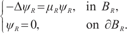
Proof   In order to prove this Lemma, we employ Kaplan's method^[7]. First we consider the case of $\theta \ne \mathrm{0},$ assume without loss generality that $\theta (\mathrm{0})=M(\theta ),$ define by $\mu (R)$ the first eigenvalue of $-\mathrm{\Delta }$ in the ball $B(R)=B_R(\mathrm{0}),$ and ${\psi }_R$ is the corresponding eigenfunction.

Thus, we have

$\{\begin{array}{l}-\mathrm{\Delta }{\psi }_R={\mu }_R{\psi }_R,\mathrm{i}\mathrm{n}{B}_R,\\ {\psi }_R=\mathrm{0},\mathrm{o}\mathrm{n}\partial B_R.\end{array}$

Assuming that ${\int }_{B_R}{\psi }_R(x)\mathrm{d}x=\mathrm{1},$ it is easy to note that $\mu (R)=\frac{{\mu }_{\mathrm{1}}}{R^{\mathrm{2}}},{\psi }_R(x)=R^{-N}{\psi }_{\mathrm{1}}(\frac{x}{R}).$

Let $B_R\subset \mathrm{\Omega },$ we set

$z(t)={\int }_{B_R}u(x,t){\psi }_R(x)\mathrm{d}x,w(t)={\int }_{B_R}v(x,t){\psi }_R(x)\mathrm{d}x,\alpha (R)={\int }_{B_R}\theta (x){\psi }_R(x)\mathrm{d}x,\beta (R)={\int }_{B_R}\vartheta (x){\psi }_R(x)\mathrm{d}x.$

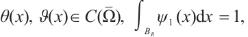Since $\theta (x),\vartheta (x)\in C(\overline{\mathrm{\Omega }}),{\int }_{B_R}{\psi }_{\mathrm{1}}(x)\mathrm{d}x=\mathrm{1},$ we obtain $\underset{R\to \mathrm{0}}{\mathrm{l}\mathrm{i}\mathrm{m}}\alpha (R)=\theta (\mathrm{0}),\underset{R\to \mathrm{0}}{\mathrm{l}\mathrm{i}\mathrm{m}}\beta (R)=\vartheta (\mathrm{0}).$

Multiplying the equations of (1)-(4) by ${\psi }_R,$integrating by parts and using Jensen inequality^[10], we have

$z_t\ge -{\mu }_{R}z+z^{p_{\mathrm{1}}}{\mathrm{e}}^{q_{\mathrm{1}}w},t>\mathrm{0},w_t\ge -{\mu }_{R}w+z^{p_{\mathrm{2}}}{\mathrm{e}}^{q_{\mathrm{2}}w},t>\mathrm{0},z(\mathrm{0})=\rho \alpha (R),w(\mathrm{0})=\rho \beta (R).$

By using the derivative formula of the product of two terms and performing simple calculations, we obtain

$({\mathrm{e}}^{{\mu }_{R}t}{z)}_t\ge {{\mathrm{e}}^{{\mu }_{R}t+}}^{q_{\mathrm{1}}w}{z}^{p_{\mathrm{1}}},({\mathrm{e}}^{{\mu }_{R}t}{w)}_t\ge {{\mathrm{e}}^{{\mu }_{R}t+}}^{q_{\mathrm{1}}w}{z}^{p_{\mathrm{2}}}.$

Integrating these inequalities over $(\mathrm{0},t),$ we see that

${\mathrm{e}}^{{\mu }_{R}t}z-\rho \alpha (R)\ge {{\int }_{\mathrm{0}}^t\left(z(s)\right)}^{p_{\mathrm{1}}}{{\mathrm{e}}^{{\mu }_{R}s+}}^{q_{\mathrm{1}}w(s)}\mathrm{d}s,{\mathrm{e}}^{{\mu }_{R}t}w-\rho \beta (R)\ge {{\int }_{\mathrm{0}}^t\left(z(s)\right)}^{p_{\mathrm{2}}}{{\mathrm{e}}^{{\mu }_{R}s+}}^{q_{\mathrm{2}}w(s)}\mathrm{d}s.$

Substituting the second inequality into the first, it follows that

$\begin{array}{l}z(t)\ge \rho \alpha (R){\mathrm{e}}^{-{\mu }_{R}t}+{\mathrm{e}}^{-{\mu }_{R}t}{{\int }_{\mathrm{0}}^t\left(z(s)\right)}^{p_{\mathrm{1}}}\mathrm{e}xp\left\{{\mu }_{R}s+q_{\mathrm{1}}\rho \beta (R){\mathrm{e}}^{-{\mu }_{R}s}+q_{\mathrm{1}}{\mathrm{e}}^{-{\mu }_{R}s}{{\int }_{\mathrm{0}}^s\left(z(y)\right)}^{p_{\mathrm{2}}}{{\mathrm{e}}^{{\mu }_{R}y+}}^{q_{\mathrm{2}}w(y)}\mathrm{d}y\right\}\mathrm{d}s\\ \ge \rho \alpha (R){\mathrm{e}}^{-{\mu }_{R}t}+{\mathrm{e}}^{{\mu }_R(s-t)}{{\int }_{\mathrm{0}}^t\left(z(\mathrm{0})\right)}^{p_{\mathrm{1}}}\mathrm{e}xp{\left\{q_{\mathrm{1}}\rho \beta (R)+q_{\mathrm{1}}{{\int }_{\mathrm{0}}^s\left(z(y)\right)}^{p_{\mathrm{2}}}\mathrm{d}y\right\}}^{{\mathrm{e}}^{-{\mu }_{{}_R}s}}\mathrm{d}s\\ \ge \rho \alpha (R){\mathrm{e}}^{-{\mu }_{R}t}+{\mathrm{e}}^{-{\mu }_{R}t}{\mathrm{e}}^{q_{\mathrm{1}}\rho \beta (R){\mathrm{e}}^{-{\mu }_{R}s}}[\rho \alpha {(R)]}^{p_{\mathrm{1}}}{\int }_{\mathrm{0}}^t\left\{\mathrm{e}xp{\left[q_{\mathrm{1}}{\int }_{\mathrm{0}}^s\left(z(y)\right)\mathrm{d}y\right]}^{{\mathrm{e}}^{-{\mu }_{{}_R}s}}\right\}\mathrm{d}s.\end{array}$

where, when $\mathrm{0}\le s\le t,$ we use the following inequality

${\mathrm{e}}^{{\mu }_R(s-t)}={\mathrm{e}}^{{\mu }_{R}s}{\mathrm{e}}^{-{\mu }_{R}t}>{\mathrm{e}}^{-{\mu }_{R}t},{\mathrm{e}}^{-{\mu }_{R}s}>{\mathrm{e}}^{-{\mu }_{R}t}.$

We fix $\mathrm{0}<\epsilon <\mathrm{1}$ and take $T_R>\mathrm{0},$ such that ${\mathrm{e}}^{-{\mu }_R{T}_R}>\mathrm{1}-\epsilon ,$ then we have

$z(t)\ge \rho \alpha (R)(\mathrm{1}-\epsilon )+(\mathrm{1}-\epsilon ){\mathrm{e}}^{q_{\mathrm{1}}\rho \beta (R)(\mathrm{1}-\epsilon )}[\rho \alpha {(R)]}^{p_{\mathrm{1}}}{\int }_{\mathrm{0}}^t\left\{\mathrm{e}\mathrm{x}\mathrm{p}{\left[q_{\mathrm{1}}{\int }_{\mathrm{0}}^s\left(z(y)\right)\mathrm{d}y\right]}^{(\mathrm{1}-\epsilon )}\right\}\mathrm{d}s.$

We set

$\begin{array}{l}H(t)=\rho \alpha (R)(\mathrm{1}-\epsilon )+(\mathrm{1}-\epsilon ){\mathrm{e}}^{q_{\mathrm{1}}\rho \beta (R)(\mathrm{1}-\epsilon )}[\rho \alpha {(R)]}^{p_{\mathrm{1}}}{\int }_{\mathrm{0}}^t\left\{\mathrm{e}\mathrm{x}\mathrm{p}{\left[q_{\mathrm{1}}{\int }_{\mathrm{0}}^s\left(z(y)\right)\mathrm{d}y\right]}^{(\mathrm{1}-\epsilon )}\right\}\mathrm{d}s,\\ H^{\text{'}}(t)=(\mathrm{1}-\epsilon )[\rho \alpha {(R)]}^{p_{\mathrm{1}}}{\mathrm{e}}^{q_{\mathrm{1}}\rho \beta (R)(\mathrm{1}-\epsilon )}\left\{\mathrm{e}\mathrm{x}\mathrm{p}{\left[q_{\mathrm{1}}{\int }_{\mathrm{0}}^s\left(z(y)\right)\mathrm{d}y\right]}^{(\mathrm{1}-\epsilon )}\right\},\\ {H^{\text{'}}}^{\text{'}}(t)={(\mathrm{1}-\epsilon )}^{\mathrm{2}}[\rho \alpha {(R)]}^{p_{\mathrm{1}}}{\mathrm{e}}^{q_{\mathrm{1}}\rho \beta (R)(\mathrm{1}-\epsilon )}\left\{\mathrm{e}\mathrm{x}\mathrm{p}{\left[q_{\mathrm{1}}{\int }_{\mathrm{0}}^s\left(z(y)\right)\mathrm{d}y\right]}^{(\mathrm{1}-\epsilon )}\right\}{q}_{\mathrm{1}}z(t).\end{array}$

Since $z(t)\ge H(t),$ we see that

$H^{\text{'}\text{'}}(t)\ge q_{\mathrm{1}}(\mathrm{1}-\epsilon )H(t)H^{\text{'}}(t).$

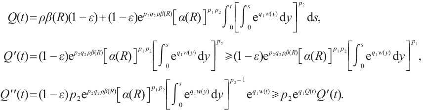
Integrating these inequalities over $(\mathrm{0},t),$ it follows that

$H^{\text{'}}(t)\ge (\mathrm{1}-\epsilon )[\rho \alpha {(R)]}^{p_{\mathrm{1}}}{\mathrm{e}}^{\rho \beta (R)(\mathrm{1}-\epsilon )}+\frac{q_{\mathrm{1}}(\mathrm{1}-\epsilon )}{\mathrm{2}}{H}^{\mathrm{2}}(t)-\frac{q_{\mathrm{1}}(\mathrm{1}-\epsilon )}{\mathrm{2}}{\rho }^{\mathrm{2}}{\left[\alpha (R)\right]}^{\mathrm{2}}{(\mathrm{1}-\epsilon )}^{\mathrm{2}}.$

Dividing the left hand side by the right hand side and integrating over $(\mathrm{0},t),$ we have

${\int }_{(\mathrm{1}-\epsilon )\rho \alpha (R)}^{H(t)}\frac{\mathrm{d}s}{(\mathrm{1}-\epsilon )[\rho \alpha {(R)]}^{p_{\mathrm{1}}}{\mathrm{e}}^{\rho \beta (R)(\mathrm{1}-\epsilon )}+\frac{q_{\mathrm{1}}(\mathrm{1}-\epsilon )}{\mathrm{2}}{s}^{\mathrm{2}}-\frac{q_{\mathrm{1}}(\mathrm{1}-\epsilon )}{\mathrm{2}}{\rho }^{\mathrm{2}}{\left[\alpha (R)\right]}^{\mathrm{2}}{(\mathrm{1}-\epsilon )}^{\mathrm{2}}}\ge t.$

We take large $\rho <\mathrm{0},$ such that

$\begin{array}{l}{T}_{\epsilon ,R}={\int }_{(\mathrm{1}-\epsilon )\rho \alpha (R)}^{\mathrm{\infty }}\frac{\mathrm{d}s}{\frac{q_{\mathrm{1}}(\mathrm{1}-\epsilon )}{\mathrm{2}}{s}^{\mathrm{2}}+(\mathrm{1}-\epsilon )[\rho \alpha {(R)]}^{p_{\mathrm{1}}}{\mathrm{e}}^{\rho \beta (R)(\mathrm{1}-\epsilon )}-\frac{q_{\mathrm{1}}{(\mathrm{1}-\epsilon )}^{\mathrm{3}}}{\mathrm{2}}{\rho }^{\mathrm{2}}{\left[\alpha (R)\right]}^{\mathrm{2}}}\\ ={\int }_{\mathrm{1}}^{\mathrm{\infty }}\frac{(\mathrm{1}-\epsilon )\rho \alpha (R)\mathrm{d}z}{\frac{q_{\mathrm{1}}{(\mathrm{1}-\epsilon )}^{\mathrm{3}}}{\mathrm{2}}{\rho }^{\mathrm{2}}{\left(\alpha (R)\right)}^{\mathrm{2}}{z}^{\mathrm{2}}+(\mathrm{1}-\epsilon )[\rho \alpha {(R)]}^{p_{\mathrm{1}}}{\mathrm{e}}^{\rho \beta (R)(\mathrm{1}-\epsilon )}-\frac{q_{\mathrm{1}}{(\mathrm{1}-\epsilon )}^{\mathrm{3}}}{\mathrm{2}}{\rho }^{\mathrm{2}}{\left[\alpha (R)\right]}^{\mathrm{2}}}\\ ={\left[\rho \alpha (R)\right]}^{-\mathrm{1}}{\int }_{\mathrm{1}}^{\mathrm{\infty }}\frac{\mathrm{d}z}{\frac{q_{\mathrm{1}}{(\mathrm{1}-\epsilon )}^{\mathrm{2}}}{\mathrm{2}}\left\{z^{\mathrm{2}}+\frac{\mathrm{2}[\rho \alpha {(R)]}^{p_{\mathrm{1}}-\mathrm{2}}{\mathrm{e}}^{\rho \beta (R)(\mathrm{1}-\epsilon )}}{q_{\mathrm{1}}{(\mathrm{1}-\epsilon )}^{\mathrm{2}}}-\mathrm{1}\right\}}.\end{array}$

Then $z$ blows up at time $T(\rho )\le T_{\epsilon ,R},$ hence we get

$\left[\rho \alpha (R)\right]T(\rho )\le {\int }_{\mathrm{1}}^{\mathrm{\infty }}\frac{\mathrm{d}z}{\frac{q_{\mathrm{1}}{(\mathrm{1}-\epsilon )}^{\mathrm{2}}}{\mathrm{2}}\left\{z^{\mathrm{2}}+\frac{\mathrm{2}[\rho \alpha {(R)]}^{p_{\mathrm{1}}-\mathrm{2}}{\mathrm{e}}^{\rho \beta (R)(\mathrm{1}-\epsilon )}}{q_{\mathrm{1}}{(\mathrm{1}-\epsilon )}^{\mathrm{2}}}-\mathrm{1}\right\}}.$

References

- Sato S. Life span of solutions with large initial data for a semilinear parabolic system[J]. Journal of Mathematical Analysis and Applications, 2011, 380(2): 632-641. [Google Scholar]
- Xu X J, Ye Z. Life span of solutions with large initial data for a class of coupled parabolic systems[J]. Zeischrift für angewamde Mathematik and physik, 2013, 64(3): 705-717. [Google Scholar]
- Zhou S, Yang Z D. Life span of solutions with large initial data for a semilinear parabolic systems[J]. Journal of Mathematical Research with Applications, 2015, 35(1): 103-109. [Google Scholar]
- Xiao F. Life span of solutions for a class of parabolic system with large initial data[J]. Acta Mathematica Scientia, 2016, 36A(4): 672-680. [Google Scholar]
- Zhou S. Life span of solutions with large initial data for a semilinear parabolic system coupling exponential reaction terms[J]. Boundary Value Problems, 2019, 154: 1-8. [Google Scholar]
- Chen H W. Global existence and blow up for a nonlinear reaction diffusion system[J]. Journal of Mathematical Analysis and Applications, 1997, 212(2): 481-492. [Google Scholar]
- Kaplan S. On the growth of solutions of quasi-linear parabolic equations[J]. Communications on Pure and Applied Mathematics, 1963, 16(3): 305-330. [Google Scholar]
- Xue Y Z. Lower bound of blow up time for solutions of a class of cross coupled porous media equations[J]. Wuhan University Journal of Natural Sciences, 2021, 26(4): 289-294. [Google Scholar]
- Leng Y, Nie Y, Zhou Q. Asymptotic behavior of solutions to a class of coupled parabolic systems[J]. Boundary Value Problems, 2019, 68: 1-11. [Google Scholar]
- Hu S Z. An interesting proof of Lebesgue theorem and Riemann inerability of functions[J]. Journal of Fuyang Teachers College (Natural Science), 2000, 17(1): 56-58(Ch). [Google Scholar]
Current usage metrics show cumulative count of Article Views (full-text article views including HTML views, PDF and ePub downloads, according to the available data) and Abstracts Views on Vision4Press platform.
Data correspond to usage on the plateform after 2015. The current usage metrics is available 48-96 hours after online publication and is updated daily on week days.
Initial download of the metrics may take a while.