| Issue |
Wuhan Univ. J. Nat. Sci.
Volume 30, Number 2, April 2025
|
|
|---|---|---|
| Page(s) | 103 - 110 | |
| DOI | https://doi.org/10.1051/wujns/2025302103 | |
| Published online | 16 May 2025 | |
Mathematics
CLC number: O175.28
Time Decay of Linearized Isentropic 2D Bipolar Navier-Stokes-Poisson System
二维线性等熵双极Navier-Stokes-Poisson方程的时间衰减
School of Mathematics, Hohai University, Nanjing 211100, Jiangsu, China
Received:
7
July
2024
Abstract
Cauchy problem for the linearized bipolar isentropic Navier-Stokes-Poisson system in  is studied. Through the reformulation of unknown functions, we change the formal system into a linearized Navier-Stokes system and a unipolar Navier-Stokes-Poisson system. Based on a delicate analysis of the corresponding Green function,
  decay estimate of the solution is obtained.
摘要
本文考虑二维空间线性等熵双极Navier-Stokes-Poisson方程的柯西问题。通过对未知函数的重组,我们把原方程组转化成线性的Navier-Stokes和单极Navier-Stokes-Poisson方程组之和。通过对相应格林函数的详细分析,得到解的 衰减估计。
衰减估计。
Key words: bipolar Navier-Stokes-Poisson system / Green function / L2 decay
关键字 : 双极Navier-Stokes-Poisson方程组 / 格林函数 / L2衰减
Cite this article: XU Hongmei, GUO Xiaoxiao. Time Decay of Linearized Isentropic 2D Bipolar Navier-Stokes-Poisson System[J]. Wuhan Univ J of Nat Sci, 2025, 30(2): 103-110.
Biography: XU Hongmei, female, Associate professor, research direction: partial differential equations. E-mail: This email address is being protected from spambots. You need JavaScript enabled to view it.
Foundation item: Supported by the National Natural Science Foundation of China (12271141)
© Wuhan University 2025
 This is an Open Access article distributed under the terms of the Creative Commons Attribution License (https://creativecommons.org/licenses/by/4.0), which permits unrestricted use, distribution, and reproduction in any medium, provided the original work is properly cited.
0 Introduction
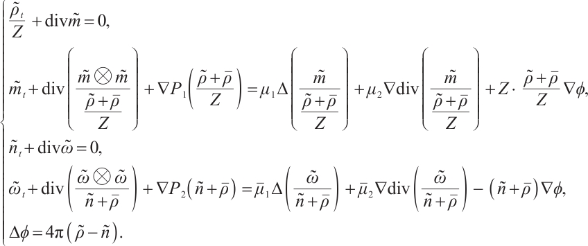
Cauchy problem of the two-dimensional bipolar Navier-Stokes-Poisson (BNSP) system has the following formulation:
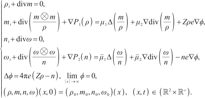 (1)
(1)
Here the unknown functions  ,
,  represent the density of ions and electrons,
  ,
,  are the momentum of ions and electrons,
  is the electrostatic potential.
  and div are the usual gradient and the divergence operator.
  ,
,  ,
,  ,
,  are constant positive viscosity coefficients. Pressure functions
  ,
,  have positive derivatives. The electrons have charge
  and the ions have charge
  where
where  ,
,  are positive constants. For simplicity, we set
  .
.
The BNSP system is used to describe the dynamics of two separate compressible fluids of ions and electrons with their self-consistent electromagnetic field. It is a hyperbolic parabolic coupling system. Because of its physical importance and mathematical challenges, there were extensive studies on the asymptotic and global existence of the BNSP system. For example, Refs. [1-5] dealt with different forms of BNSP, and got the global existence of classical solution and its decay. But most results are about space dimension  . There are few results about space
  . This paper studies
  decay estimate of a linearized two-dimensional BNSP system.
Throughout this paper,  denotes the Lebesgue integrable space function,
  means the Sobolev space function.
  denote some general positive constants.
1 Reformulation and Linearization
Suppose the initial value  of (1) tends to equilibrium state
  as
as  Set
Set  ,
, ,
, ,
, . Then (1) can be rewritten as
 (2)
(2)
System (2) can be reformulated as a linear part plus a nonlinear part.
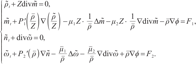 (3)
(3)
The left side of (3) is the linearized part of (2) near  , and the right side of (3) is the nonlinearized part. For simplicity, we denote the perturbation
  ,
,  ,
,  ,
,  as
as  ,
, ,
, ,
, , so the linearized system of (1) near the state
  is
is
 (4)
(4)
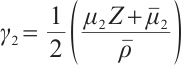
where 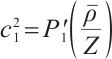 ,
,  .
.
Our final result in this paper is the following theorem.
Theorem 1 If the initial data  ,
,  ,
,  we have the following estimate:

If  , for any positive
  , we have
  ,
,

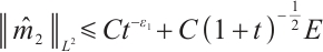
Further on, if  , for any positive
  , we have
  ,
,  .
.
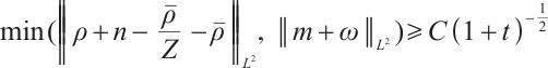
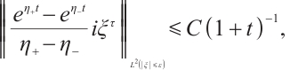
Remark 1 From Theorem 1, the perturbation of the sum of density and momentum decay at the rate  , the perturbation of the difference of density decay at the rate
  , but the difference of momentum hardly decay at
  because of the influence of the electronic field. Due to the low decay rate, it is difficult to go on the global existence of the system.
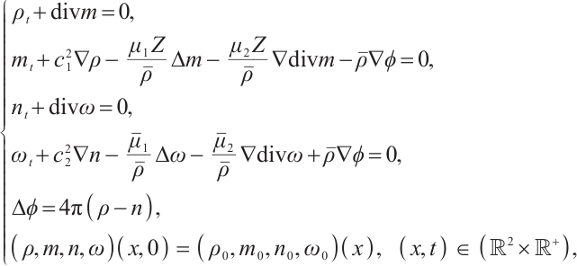
We want to separate system (4) into several small sets of equations. Considering the fifth equation of (4), we denote  ,
,  ,
,  ,
, 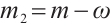 , (4) is equal to the following system:
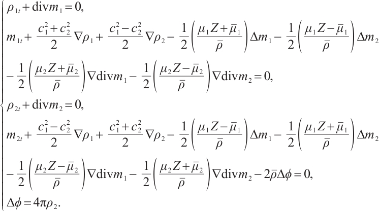 (5)
(5)
For simplicity, we suppose  ,
,  ,
,  , denote
 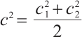 ,
,  ,
,  . System (5) can be separated into the following two systems
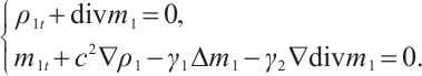 (6)
(6)
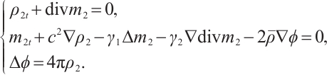 (7)
(7)
We find that (6) is a linearized isentropic Navier-Stokes (NS) system while (7) is a linearized unipolar Navier-Stokes-Poisson (NSP) system. We study them respectively in the next step.
2
 Decay of Linearized NS System
If the initial data of (6) is 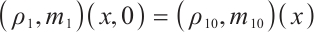 , according to (1.3) in Ref. [6], we have
 (8)
(8)
where  is a
is a  unit matrix,
 (9)
(9)
From (9), when  is small enough, there is no problem with the decay estimate for the Green function; when
  is bounded and away from zero,
  may tend to zero, so we need to consider the integrability of the Green function; when
  is large enough, for example,
 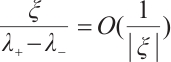 has no
  bounds. Next, we will divide frequency into three different parts and will use different methods to consider the decay rate respectively.
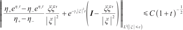
When 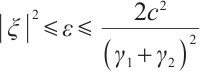 , we have

We find the construction of  is like that of
  in Ref. [7]. Initiated by the estimation method in Ref. [7], we get
Similarly
Thus
 (10)
(10)
Using the same method, we can get
 (11)
(11)
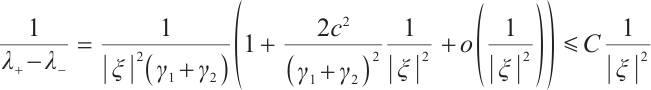
When  , there exist positive constant
  such that
  .
.
Because  ,
,  are smooth functions, we can easily get
 (12)
(12)
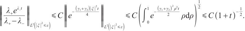
When  , notice
  for some positive
  , then
we have
 (13)
(13)
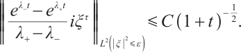
Next, we consider 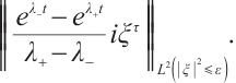
Since  we have
then
 (14)
(14)
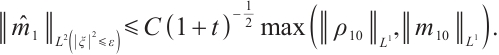
From (9) and (14), we have
 (15)
(15)
If we fix 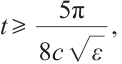 we have
 (16)
(16)
 (17)
(17)
From (15), (16), and (17) , when  is large enough, we have
 (18)
(18)
From (8) and (18), we have
 (19)
(19)
 (20)
(20)
Together with (8), (10), (11), (12), (13), (19), and (20), we get our results.
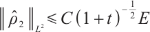
Theorem 2 Suppose 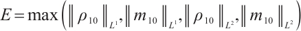 , there exists a positive constant
  such that max
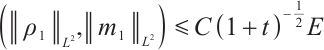 . Further on, when
  is large enough, we have
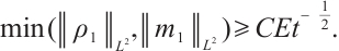
Remark 2 From Theorem 2, we know our decay estimate about  is optimal.
3
 Decay of Linearized NSP System
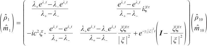
Suppose the initial data of (7) is  , using the method of Ref. [8], the solution of (7) can be expressed as
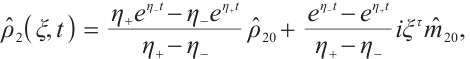 (21)
(21)
 (22)
(22)
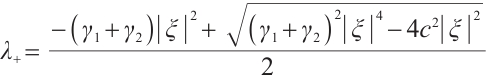
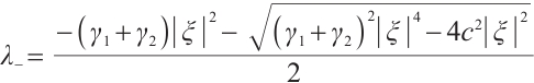
where
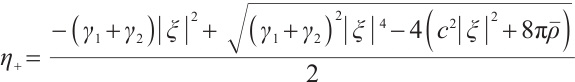
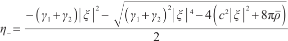 (23)
(23)
When  , and
, and  is small enough, we have
 (24)
(24)
then
Similarly
 (25)
(25)
 (26)
(26)
 (27)
(27)
From (21), (25), and (26), we have
 (28)
(28)
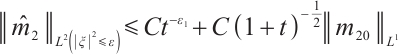
But for 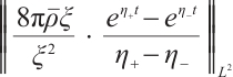 , we need a much more delicate analysis.
If 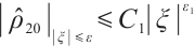 , for any positive
  , from (22) and (24), we have
 (29)
(29)
From (22), (26), (27) and (29), if  , for any positive
  , we have
 (30)
(30)
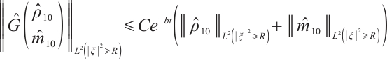
when  ,
,  with
with  large enough, using the same method as that of (11), and (12), we can also get
 (31)
(31)
 (32)
(32)
Together with (28), (30), (31) and (32), we have
Theorem 3 Suppose 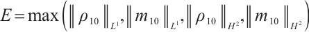 ,
,  for any positive
  , there exists a positive constant
  such that
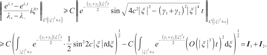
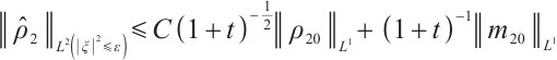
Theorem 4 If 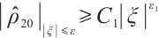 , for any positive
  , we have
 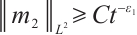 ,
, 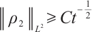 .
.
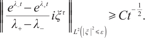
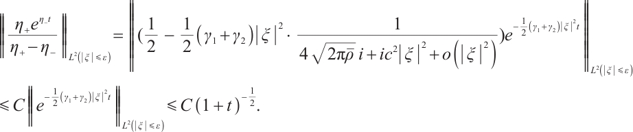
Proof From (23) and (24), we have
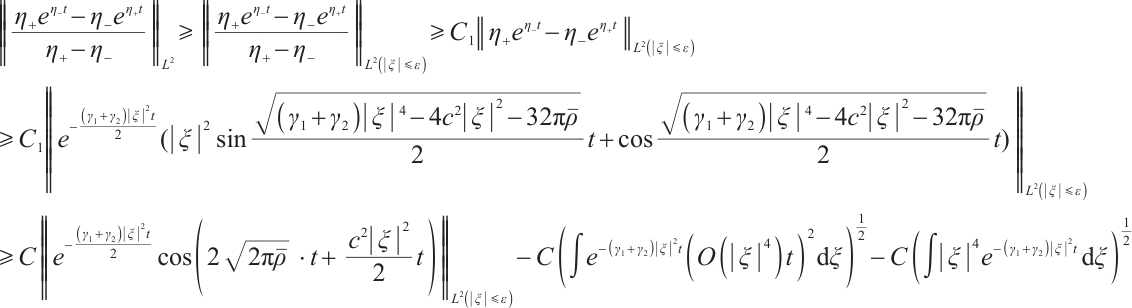
 (33)
(33)
Fix t large enough,
 (34)
(34)
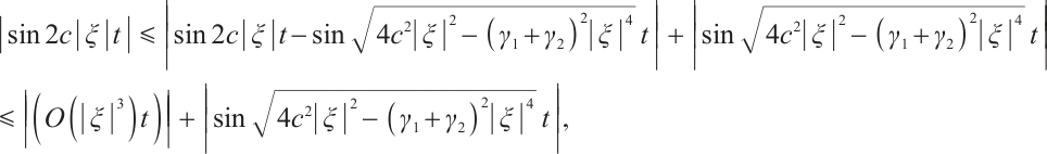
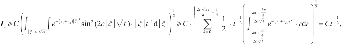
Because
 (35)
(35)
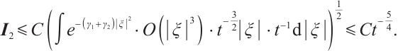
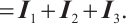
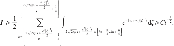
from (33), (34) and (35), we have
 (36)
(36)
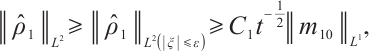
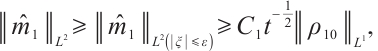
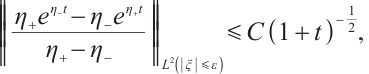
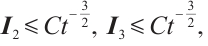
Similarly, we have
 (37)
(37)
Together with (21), (22), (36) and (37), we get our results.
Considering the meaning of  ,
,  ,
,  ,
,  , combining Theorem 2, Theorem 3, and Theorem 4, we have the conclusion of Theorem 1 in this paper.
References
- Li H L, Yang T, Zou C. Time asymptotic behavior of the bipolar Navier-Stokes-Poisson system[J]. Acta Mathematica Scientia, 2009, 29(6): 1721-1736. [Google Scholar]
- Wu Z G, Wang W K. Space-time estimates of the 3D bipolar compressible Navier-Stokes-Poisson system with unequal viscosities[J]. Science China Mathematics, 2024, 67(5): 1059-1084. [Google Scholar]
-
Zhang G J, Li H L, Zhu C J. Optimal decay rate of the non-isentropic compressible Navier-Stokes-Poisson system in
 3[J]. Journal of Differential Equations, 2011, 250(2): 866-891.
[Google Scholar]
3[J]. Journal of Differential Equations, 2011, 250(2): 866-891.
[Google Scholar]
- Lin Q Y, Hao C C, Li L H. Global well-posedness of compressible bipolar Navier-Stokes-Poisson equations[J]. Acta Mathematica Sinica, 2012, 28 (5): 925-940. [Google Scholar]
- Zhao Z Y, Li Y P. Global existence and optimal decay rate of the compressible bipolar Navier-Stokes-Poisson equations with external force[J]. Nonlinear Analysis: Real World Applications, 2014, 16: 146-162. [Google Scholar]
- Xu H M, Wang W K. Pointwise estimate of solutions of isentropic Navier-Stokes equations in even space-dimensions[J]. Acta Mathematica Scientia, 2001, 21(3): 417-427. [Google Scholar]
- Xu H M, Yan L X. L2 decay estimate of BCL equation[J]. Wuhan Univ J of Nat Sci, 2017, 22(4): 283-288. [Google Scholar]
- Li H L, Zhang T. Large time behavior of solutions to 3D compressible Navier-Stokes-Poisson system[J]. Science China Mathematics, 2012, 55: 159-177. [Google Scholar]
Current usage metrics show cumulative count of Article Views (full-text article views including HTML views, PDF and ePub downloads, according to the available data) and Abstracts Views on Vision4Press platform.
Data correspond to usage on the plateform after 2015. The current usage metrics is available 48-96 hours after online publication and is updated daily on week days.
Initial download of the metrics may take a while.