| Issue |
Wuhan Univ. J. Nat. Sci.
Volume 30, Number 2, April 2025
|
|
|---|---|---|
| Page(s) | 150 - 158 | |
| DOI | https://doi.org/10.1051/wujns/2025302150 | |
| Published online | 16 May 2025 | |
Mathematics
CLC number: TP13
Modified Fixed-Time Synchronization Criteria of Complex Networks with Time-Varying Delays via Continuous or Discontinuous Control
基于连续或不连续控制的时变时滞复杂网络的修正固定时间同步判据
School of Mathematics and Statistics, Hubei Normal University, Huangshi 435002, Hubei, China
† Corresponding author. E-mail: hbnuwu@yeah.net
Received:
10
February
2024
This paper investigates modified fixed-time synchronization (FxTS) of complex networks (CNs) with time-varying delays based on continuous and discontinuous controllers. First, for the sake of making the settling time (ST) of FxTS is independent of the initial values and parameters of the CNs, a modified fixed-time (FxT) stability theorem is proposed, where the ST is determined by an arbitrary positive number given in advance. Then, continuous controller and discontinuous controller are designed to realize the modified FxTS target of CNs. In addition, based on the designed controllers, CNs can achieve synchronization at any given time, or even earlier. And control strategies effectively solve the problem of ST related to the parameters of CNs. Finally, an appropriate simulation example is conducted to examine the effectiveness of the designed control strategies.
摘要
本文基于连续和不连续控制器,研究了带有时变时滞的复杂网络的修正固定时间同步。首先,为了保证固定时间同步的确定时间与复杂网络的初始值和参数都无关,提出了一个修正的固定时间稳定性定理,其中确定时间是由提前给定的任意正数决定。然后,设计了连续控制器和不连续控制器,用于实现复杂网络的固定时间同步目标。基于所设计的控制器,复杂网络可以在任意给定时间甚至更早实现同步。并且控制策略有效解决了确定时间与复杂网络参数有关的问题。最后通过仿真实例验证了所设计控制策略的有效性。
Key words: complex networks / settling time / fixed-time synchronization / controllers / time-varying delays
关键字 : 复杂网络 / 确定时间 / 固定时间同步 / 控制器 / 时变时滞
Cite this article: WU Huan, WU Ailong, ZHANG Jin’e. Modified Fixed-Time Synchronization Criteria of Complex Networks with Time-Varying Delays via Continuous or Discontinuous Control[J]. Wuhan Univ J of Nat Sci, 2025, 30(2): 150-158.
Biography: WU Huan, female, Master candidate, research direction: synchronization and control of complex network. E-mail: 2822371594@qq.com
Foundation item: Supported by the National Natural Science Foundation of China (62476082)
© Wuhan University 2025
 This is an Open Access article distributed under the terms of the Creative Commons Attribution License (https://creativecommons.org/licenses/by/4.0), which permits unrestricted use, distribution, and reproduction in any medium, provided the original work is properly cited.
0 Introduction
Complex networks (CNs) have attracted increasing attention in many fields, for examples, social networks[1], electrical power networks[2], biological networks and aviation networks, etc[3-4]. Synchronization is an important issue in CNs and has been extensively studied in recent years, such as asymptotic synchronization[5-6], and exponential synchronization[7-8]. Asymptotic synchronization of CNs with structure uncertainty is solved in Ref.[9]. In Ref.[10], exponential synchronization is realized by proposing a sampled data controller for complex dynamical networks. However, asymptotic and exponential synchronization are achieved when time tends to infinity, which leads a lot of wasted resources in practical applications.
In order to achieve synchronization of CNs as fast as possible, researchers have proposed finite-time synchronization (FnTS) strategy, and FnTS of various neural networks has been well-studied[11-13]. Refs.[14] and [15] studied FnTS of dynamical networks with several weights, which provides a better description of actual networks. FnTS of memristive dynamical networks and finite-time (FnT) stability of singular dynamical networks with time delays are considered in Refs.[16] and [17], respectively. Notably, the settling time (ST) of FnTS depends on the initial values of the considered neural networks. However, since these initial values are generally unknown or even unavailable in practical networks, the exact ST remains theoretically indeterminable.
Therefore, for the purpose of obtaining the ST when the initial values of the neural networks are unknown, the strategy of fixed-time synchronization (FxTS) is introduced by Polyakov[18]. And since the ST of the FxTS is independent of the initial values, FxTS strategy has a wider range of applications than FnTS. In recent yesrs, FxTS has been widely used in communication security[19-20], bioengineering[21-22], and financial transaction[23]. FxTS of coupled neural networks was studied in Ref.[24], where the case of dynamical networks containing discontinuous activation and mismatched parameter is considered. Ref.[25] discussed FxTS of drive and response networks with noise disturbances and discontinuous nodes, and this model can well simulate the workings of neurons and solve some bioengineering problems. Fixed-time (FxT) group consensus on dynamical networks with multiple nodes was studied in Ref.[26], and the implementation of FxT group consensus can greatly increase the security of communication. In these papers and Ref.[27], the ST of FxTS are all determined by the disturbed parameters regardless of the initial values of the neural networks. However, the parameters of the neural networks are usually uncertain due to the presence of some perturbations. Therefore, it is a challenge to achieve FxTS, where the ST is independent of the initial values and disturbed parameters.
In addition, as a tool for achieving FxTS, continuous and discontinuous controllers are often used. Refs.[28] and [29] explored FxT synchronous behaviour of CNs by continuous controllers, which can effectively avoid chattering during the synchronization process. Ref.[30] addressed the FxTS of coupled CNs with delays under the discontinuous controllers, where the controllers contain the symbolic functions.
Through the above statements, it is easy to find that FxTS of CNs without time delays has been fully investigated in Refs.[20-27, 29]. But as we all know, time delays, especially time-varying delays, are unavoidable in engineering applications because of the delayed response of the neural networks and the limited speed of signal propagation. Numerous studies have investigated the synchronization of CNs with time delays[31-32]. In Refs.[33] and [34], global exponential synchronization and asymptotic exponential synchronization of CNs with time-delay were investigated by designing controllers, respectively. In Ref.[35], FxTS of CNs with time-varying delays was achieved, where the ST was determined by the turbulent parameters of the considered networks and the controller was complicated. Moreover, few studies have investigated FxTS in CNs with time-varying delays whose ST remains unaffected by network parameters.
This paper aims to explore FxTS of CNs with time-varying delays via continuous or discontinuous control. The key contributions of this paper are given below: (1) Suitable continuous and discontinuous controllers are constructed for implementing FxTS of CNs, and the controllers given in this paper may be simpler than those in the existing literatures [27-30, 35]. (2) In contrast to the existing result [35], this paper achieves true FxTS. In other words, the ST is independent of the initial values and the parameters of the considered networks.
The remainder of this paper is arranged as follows. Section 1 presents the model of CNs and preliminaries. Some control strategies are provided for FxTS of CNs in Section 2. A simulation example is formulated in Section 3. Finally, Section 4 gives the conclusion.
1 Model Description and Preliminaries
Let  and
and  represent the sets of real numbers and nonnegative real numbers, respectively.
  means the
  dimensional real space equipped with the Euclidean norm
  .
.  is the maximum eigenvalue of matrix
  . The notations
  denotes sign function.
  means the Kronecker product.
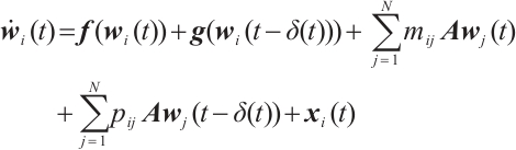
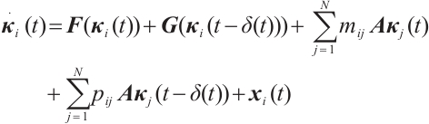
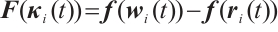
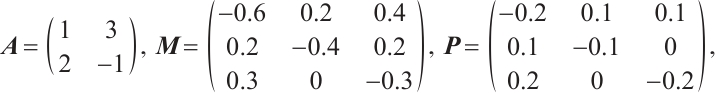
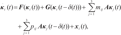
Consider a class of CNs with time-varying delays whose modle is formulated as:
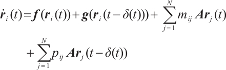
with initial condition
where  denotes neuron state vector,

are nonlinear vector functions.  is the time-varying delays and meets
  .
.  is the internal coupling matrix.
  and
and  are the coupling configuration matrices. Suppose there is a connection between nodes
  and
and  , then
  , otherwise,
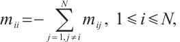
  , and the diagonal elements of matrix
  and
and  are defined by
The controlled CNs corresponding to (1) can be described as below:
with initial condition
where  is the state vector and
  denotes the appropriate controller.
Define an error vector  ,
,  . Then the synchronization error neural networks can be expressed as
with initial condition

where

Assumption 1 For  , there are positive constants
  and
and  such that


Definition 1 (FnT Stability[24]) For a class of neural network
where  is the neural network parameter.
The trivial solution  of neural network (4) is said to be globally FnT stable, if it satisfies globally stable and
  for
for  , where
  is called ST function.
Definition 2 (FxT Stability[28]) For neural network (4), the trivial solution  is globally FxT stable, if it meets globally FnT stable and
  , subject to the ST function
  for
for  .
.
Remark 1 In Definition 1, neural network (4) achieves FnT stabilization at  , and the ST function
  is connected to the initial value
  of (4). In Definition 2, neural network (4) achieves FxT stabilization at
  , and
, and  is associated with the parameters
  of neural network (4).
Definition 3 (Modified FxT Stability[35]) For neural network (4), the trivial solution  is called modified FxT stable, if it meets globally FnT stable and for
  (
( is arbitrarily given positive number in advance), subject to the ST function
  for
for  .
.
Remark 2 It is clear that Definition 3 is not the same as Definition 1 and Definition 2. In Definition 3,  is an arbitrary positive value given in advance, which is unrelated to the initial value and the parameter of neural network (4). Thus, the ST in Definition 3 is also irrelevant to the initial values and parameters.
Lemma 1[29] Given  and
and  , then
Lemma 2[36] Suppose there exists the Lyapunov function  such that

where  ,
,  . Then the trivial solution of neural network (4) is globally FnT stable, and for any given
  ,
,  fulfils the inequality as follows:

and  ,
,  , where the ST function
  is given below
Lemma 3 Suppose there exists the Lyapunov function  such that
then the trivial solution of neural network (4) is modified globally FxT stable, that is  and
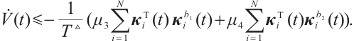
and  satisfies the inequality as following T≤
 , where
  ,
,  ,
,  ,
,  , and
, and  >0 is a predetermined arbitrary time.
Proof Define the function  , then

As  ,
,  , then
  and
and  , and based on Lemma 2, the trivial solution of (4) is globally FnT stable.
Combining (5), we can obtain  so
so
Note that  ,
,  , one may have

Define  , then
Without loss of generality, we consider two possible cases as follows:
(i) When 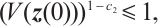
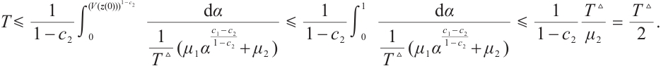
(ii) When 
By definition of  , we can deduce that
From (i) and (ii), we have T≤ . The proof is completed.
Remark 3 In Lemma 3, if there exist positive numbers  and
and  such that
  ,
,  (or
(or  ). Then, the trivial solution of (4) is globally FxT stable, and
  .
.
2 Theoretical Results
In this section, the strategies of continuous and discontinuous control are provided for achieving the modified FxTS of CNs (1) and (2), respectively.
2.1 Modified FxTS with Continuous Controller
Theorem 1 Under Assumption 1, the continuous controller is

then CNs (1) and (2) can achieve modified FxTS, and the ST is  where
where


Proof We define the nonegative function as follows:

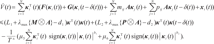
Based on Assumption 1 and the synchronization error neural network (3), one can calculate that
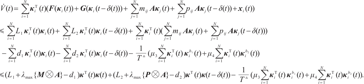
As one gets
From Lemma 1, it can easily obtain that

and

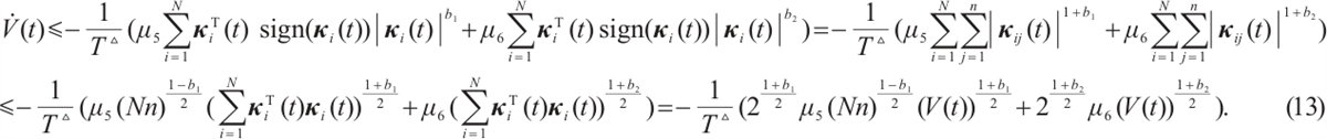
Using (8) and (9) in (7) leads to

When taking 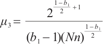 and
and 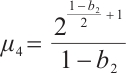 , we obtain from (10) that

If  and
and  , the following inequality is the direct result of (11),

where  ,
,  .
.
So, based on Lemma 3, the synchronization error neural networks (3) is modified FxT stable, and  . That is, CNs (1) and (2) are modified FxTS via continuous controller (6). The proof is completed.
Remark 4 Based on the conditions given in Theorem 1, when  ,
,  (or
(or  ), CNs (1) and (2) can also achieve modified FxTS, and T≤
 .
.
2.2 Modified FxTS with Discontinuous Controller
Theorem 2 Under Assumption 1, the discontinuous controller is given by

then CNs (1) and (2) can realize modified FxTS, and T≤ , where
Proof Define a nonegative function 
Similar to Theorem 1, we can find
As  and based on Lemma 1, then
Based on (10), it follows from  and
and  that
that
The following proof is identical to Theorem 1, so it is omitted here. As a result, CNs (1) and (2) are modified FxTS via discontinuous controller (12). The proof is completed.
Remark 5 On the basis of the conditions given in Theorem 2, when  ,
,  (or
(or  ), CNs (1) and (2) are modified FxTS, and
  .
.
Remark 6 In this paper, the controller (6) and (12) contain linear terms  and
and  , and based on
  ,
,  and Lemma 3, CNs (1) and (2) can realize modified FxTS at ST
  , before any given time
  . Although the value of
  and
and  are related to
  , the ST obtained is unrelated to the initial values and disturbed parameters of error neural networks (3), so it is more useful compared with the existing results[24, 28].
3 A Simulation Example
At last, an appropriate simulation example is given to confirm the effectiveness and feasibility of the strategies of continuous and discontinuous control.
We consider the following CNs with three identical nodes:

where  ,
,  ,
,


The controlled CNs corresponding to (15) can be described as:

where  ,
,  is the controller.
Consequently, the error dynamical networks are given by:
where


From Assumption 1, we can obtain that  ,
,  . Let
. Let  ,
,  ,
,  ,
,  ,
,  ,
,  , it is easy to see that these conditions satisfy Theorem 1 and Theorem 2.
Next, this study prove the validity of the control strategies. The initial values of CNs (15) for simulation are chosen as 
The initial values of CNs (16) are chosen as
Based on the initial values of CNs (15) and (16) given above, the simulation results are presented in Figs. 1-3. Figure 1 simulates the evolution of error dynamical networks (17) without controller. It shows error dynamical networks (17) cannot converge to zero which means CNs (15) and (16) are not synchronized. When  =0.1, Figure 2 gives the evolution of error dynamical networks (17) under continuous controller (6), and the ST
  is
is  . The evolution of error dynamical networks (17) under discontinuous controller (12) is given in Fig. 3, and the ST
  is
is  . From Figs. 2 and 3, it is not difficult to see that the CNs (15) and (16) can achieve synchronization. This shows that the control strategies proposed in this paper are effective.
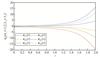 |
Fig. 1 The error networks (17) without controller |
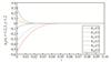 |
Fig. 2 The error networks (17) with controller (6) |
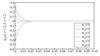 |
Fig. 3 The error networks (17) with controller (12) |
4 Conclusion
In this paper, based on continuous and discontinuous control strategies, modified FxTS criteria of CNs with time-varying delays have been addressed, where the ST is determined by an arbitrary positive number given in advance, so the ST is not correlated with either the initial value or the parameters of the CNs. An appropriate simulation example is provided to show the effectiveness of the strategies of continuous and discontinuous control. Further investigation may aim to design the controller for modified FxTS of impulsive CNs.
References
- Bandyopadhyay A, Kar S. Coevolution of cooperation and network structure in social dilemmas in evolutionary dynamic complex network[J]. Applied Mathematics and Computation, 2018, 320: 710-730. [Google Scholar]
- Rohden M, Sorge A, Timme M, et al. Self-organized synchronization in decentralized power grids[J]. Physical Review Letters, 2012, 109(6): 064101. [CrossRef] [PubMed] [Google Scholar]
- Xing W, Shi P, Agarwal R K, et al. A survey on global pinning synchronization of complex networks[J]. Journal of the Franklin Institute, 2019, 356(6): 3590-3611. [Google Scholar]
- Wang Y Q, Lu J Q, Liang J L, et al. Pinning synchronization of nonlinear coupled lur’e networks under hybrid impulses[J]. IEEE Transactions on Circuits and Systems II: Express Briefs, 2019, 66(3): 432-436. [Google Scholar]
- Liao H Y, Zhang Z Q. Global asymptotic synchronization for coupled heterogeneous complex networks via Laplace transform approach[J]. Journal of Applied Mathematics and Computing, 2024, 70(4): 2743-2766. [Google Scholar]
- Xu Y, Huang Z B, Rao H X, et al. Quasi-synchronization for periodic neural networks with asynchronous target and constrained information[J]. IEEE Transactions on Systems, Man, and Cybernetics: Systems, 2021, 51(7): 4379-4388. [Google Scholar]
- Qin J H, Gao H J, Zheng W X. Exponential synchronization of complex networks of linear systems and nonlinear oscillators: A unified analysis[J]. IEEE Transactions on Neural Networks and Learning Systems, 2015, 26(3): 510-521. [Google Scholar]
- Wan X X, Yang X S, Tang R Q, et al. Exponential synchronization of semi-Markovian coupled neural networks with mixed delays via tracker information and quantized output controller[J]. Neural Networks, 2019, 118: 321-331. [Google Scholar]
- Li L X, Kurths J, Peng H P, et al. Exponentially asymptotic synchronization of uncertain complex time-delay dynamical networks[J]. The European Physical Journal B, 2013, 86(4): 125. [Google Scholar]
- Wu Z G, Park J H, Su H Y, et al. Exponential synchronization for complex dynamical networks with sampled-data[J]. Journal of the Franklin Institute, 2012, 349(9): 2735-2749. [Google Scholar]
- Bhat S P, Bernstein D S. Finite-time stability of continuous autonomous systems[J]. SIAM Journal on Control and Optimization, 2000, 38(3): 751-766. [Google Scholar]
- Yang X S, Ho D W C, Lu J Q, et al. Finite-time cluster synchronization of T-S fuzzy complex networks with discontinuous subsystems and random coupling delays[J]. IEEE Transactions on Fuzzy Systems, 2015, 23(6): 2302-2316. [Google Scholar]
- Li D K, Wei X M. Finite-time generalized synchronization and parameter identification of chaotic systems with different dimensions[J]. Wuhan University Journal of Natural Sciences, 2022, 27(2): 135-141. [Google Scholar]
- Wang J L, Xu M, Wu H N, et al. Finite-time passivity of coupled neural networks with multiple weights[J]. IEEE Transactions on Network Science and Engineering, 2018, 5(3): 184-197. [Google Scholar]
- Wang J L, Zhang X X, Wu H N, et al. Finite-time passivity and synchronization of coupled reaction-diffusion neural networks with multiple weights[J]. IEEE Transactions on Cybernetics, 2019, 49(9): 3385-3397. [Google Scholar]
- Gong S Q, Guo Z Y, Wen S P, et al. Finite-time and fixed-time synchronization of coupled memristive neural networks with time delay[J]. IEEE Transactions on Cybernetics, 2021, 51(6): 2944-2955. [Google Scholar]
- Yang X Y, Li X D, Cao J D. Robust finite-time stability of singular nonlinear systems with interval time-varying delay[J]. Journal of the Franklin Institute, 2018, 355(3): 1241-1258. [Google Scholar]
- Polyakov A. Nonlinear feedback design for fixed-time stabilization of linear control systems[J]. IEEE Transactions on Automatic Control, 2012, 57(8): 2106-2110. [Google Scholar]
- Alimi A M, Aouiti C, Abed Assali E. Finite-time and fixed-time synchronization of a class of inertial neural networks with multi-proportional delays and its application to secure communication[J]. Neurocomputing, 2019, 332: 29-43. [Google Scholar]
- Zhou L L, Tan F, Li X H, et al. A fixed-time synchronization-based secure communication scheme for two-layer hybrid coupled networks[J]. Neurocomputing, 2021, 433: 131-141. [Google Scholar]
- Zhang W L, Li C D, Huang T W, et al. Fixed-time synchronization of complex networks with nonidentical nodes and stochastic noise perturbations[J]. Physica A: Statistical Mechanics and Its Applications, 2018, 492: 1531-1542. [Google Scholar]
- Tan F, Zhou L L, Yu F, et al. Fixed-time continuous stochastic synchronisation of two-layer dynamical networks[J]. International Journal of Systems Science, 2020, 51(2): 242-257. [Google Scholar]
- He Y J, Peng J, Zheng S. Fractional-order financial system and fixed-time synchronization[J]. Fractal and Fractional, 2022, 6(9): 507. [Google Scholar]
- Li N, Wu X Q, Feng J W, et al. Fixed-time synchronization of coupled neural networks with discontinuous activation and mismatched parameters[J]. IEEE Transactions on Neural Networks and Learning Systems, 2021, 32(6): 2470-2482. [Google Scholar]
- Li N, Wu X Q, Feng J W, et al. Fixed-time synchronization in probability of drive-response networks with discontinuous nodes and noise disturbances[J]. Nonlinear Dynamics, 2019, 97(1): 297-311. [Google Scholar]
- Shang Y L. Fixed-time group consensus for multi-agent systems with non-linear dynamics and uncertainties[J]. IET Control Theory & Applications, 2018, 12(3): 395-404. [Google Scholar]
- Xu Y H, Wu X Q, Li N, et al. Fixed-time synchronization of complex networks with a simpler nonchattering controller[J]. IEEE Transactions on Circuits and Systems II: Express Briefs, 2020, 67(4): 700-704. [Google Scholar]
- Xu Y H, Wu X Q, Mao B, et al. Fixed-time synchronization in the pth moment for time-varying delay stochastic multilayer networks[J]. IEEE Transactions on Systems, Man, and Cybernetics: Systems, 2022, 52(2): 1135-1144. [Google Scholar]
- Zhang W L, Yang X S, Li C D. Fixed-time stochastic synchronization of complex networks via continuous control[J]. IEEE Transactions on Cybernetics, 2019, 49(8): 3099-3104. [Google Scholar]
- Lü H, He W L, Han Q L, et al. Fixed-time synchronization for coupled delayed neural networks with discontinuous or continuous activations[J]. Neurocomputing, 2018, 314: 143-153. [Google Scholar]
- Guo B B, Shi P, Zhang C P. Aperiodically intermittent control for synchronization of stochastic coupled networks with semi-Markovian jump and time delays[J]. Nonlinear Analysis: Hybrid Systems, 2020, 38: 100938. [Google Scholar]
- Guo X X, Xia J W, Shen H, et al. Synchronization of time-delayed complex networks with delay-partitioning: A Chua’s circuit networks application[J]. Journal of the Franklin Institute, 2023, 360(18): 14208-14221. [Google Scholar]
- Yang X S, Li X D, Lu J Q, et al. Synchronization of time-delayed complex networks with switching topology via hybrid actuator fault and impulsive effects control[J]. IEEE Transactions on Cybernetics, 2020, 50(9): 4043-4052. [Google Scholar]
- Liu Y R, Wang Z D, Liang J L, et al. Synchronization and state estimation for discrete-time complex networks with distributed delays[J]. IEEE Transactions on Systems, Man, and Cybernetics Part B, Cybernetics: A Publication of the IEEE Systems, Man, and Cybernetics Society, 2008, 38(5): 1314-1325. [Google Scholar]
- Hu J T, Sui G X, Li X D. Fixed-time synchronization of complex networks with time-varying delays[J]. Chaos, Solitons & Fractals, 2020, 140: 110216. [Google Scholar]
- Xu Z L, Li X D, Duan P Y. Synchronization of complex networks with time-varying delay of unknown bound via delayed impulsive control[J]. Neural Networks, 2020, 125: 224-232. [Google Scholar]
All Figures
|
Fig. 1 The error networks (17) without controller |
| In the text | |
|
Fig. 2 The error networks (17) with controller (6) |
| In the text | |
|
Fig. 3 The error networks (17) with controller (12) |
| In the text | |
Current usage metrics show cumulative count of Article Views (full-text article views including HTML views, PDF and ePub downloads, according to the available data) and Abstracts Views on Vision4Press platform.
Data correspond to usage on the plateform after 2015. The current usage metrics is available 48-96 hours after online publication and is updated daily on week days.
Initial download of the metrics may take a while.