| Issue |
Wuhan Univ. J. Nat. Sci.
Volume 30, Number 2, April 2025
|
|
|---|---|---|
| Page(s) | 159 - 168 | |
| DOI | https://doi.org/10.1051/wujns/2025302159 | |
| Published online | 16 May 2025 | |
Mathematics
CLC number: O221
A Full-Newton Step Interior-Point Algorithm Based on a New Search Direction for P*(κ)-Linear Complementarity Problem
基于新搜索方向求解P*(κ)-线性互补问题的全牛顿步内点算法
1
Department of Mathematics, Anhui Institute of Information Technology, Wuhu 241000, Anhui, China
2
College of Science, China Three Gorges University, Yichang 443002, Hubei, China
† Corresponding author. E-mail: This email address is being protected from spambots. You need JavaScript enabled to view it.
Received:
15
July
2024
Abstract
In this paper, a full-Newton step interior-point algorithm is proposed for solving  -linear complementarity problem based on a new search direction, which is an extension of Grimes' algorithm. It is proved that the number of iterations of the algorithm is
  , which matches the best known iteration bound of the interior-point method for
  -linear complementarity problem. Some numerical results have proved the feasibility and efficiency of the proposed algorithm.
摘要
为了求解 -线性互补问题,本文提出了一种基于新搜索方向的全牛顿内点算法。此算法是 Grimes 算法的扩展。研究证明,该算法的迭代次数为
 ,与已知的求解
 -线性互补问题的最佳迭代复杂度一致。一些数值结果证明了所提出的算法的可行性和有效性。
Key words: full-Newton step / interior-point method / P*(κ)-linear complementarity problem / polynomial complexity
关键字 : 全牛顿步 / 内点算法 / P*(κ)-线性互补问题 / 多项式复杂性
Cite this article: WANG Li, ZHANG Mingwang. A Full-Newton Step Interior-Point Algorithm Based on a New Search Direction for P* (κ)-Linear Complementarity Problem[J]. Wuhan Univ J of Nat Sci, 2025, 30(2): 159-168.
Biography: WANG Li, female, Lecturer, research direction: optimization theory and algorithm. E-mail: This email address is being protected from spambots. You need JavaScript enabled to view it.
Foundation item: Supported by the Optimization Theory and Algorithm Research Team (23kytdzd004), the General Programs for Young Teacher Cultivation of Educational Commission of Anhui Province of China (YQYB2023090) and the University Science Research Project of Anhui Province (2024AH050631)
© Wuhan University 2025
 This is an Open Access article distributed under the terms of the Creative Commons Attribution License (https://creativecommons.org/licenses/by/4.0), which permits unrestricted use, distribution, and reproduction in any medium, provided the original work is properly cited.
0 Introduction
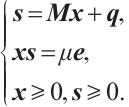
In this paper, we consider the linear complementarity problem (LCP) in the standard form
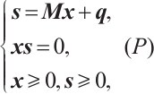
where  and
and  denotes the componentwise product (Hadamard product) of the vectors
  and
and  . The LCP has many applications in science, engineering, economics and operations research[1].
The problem (P) is called  -LCP if
  is a
is a  matrix, i.e., there exists a constant
  such that for every
  ,
,
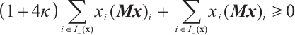
where  In particular, when
  -LCP reduces to be monotone LCP (MLCP), which includes linear programming (LP) and convex quadratic programming (CQP) as special cases.
To introduce our method for solving  -LCP, we first review the primal-dual interior-point method (IPM), which has proven to be one of the most efficient IPMs. The primal-dual IPM for LP was first introduced by Kojima et al in 1989[2] and extended to a wider class of problems such as semidefinite programming (SDP)[3], second order cone programming (SOCP)[4], and LCP[5]. It is known that the main feature of the primal-dual IPM is to approximately follow the central path, so the existence of the central path is crucial. Kojima et al[6] first proved the existence of the central path for
  -LCP and generalized the primal-dual IPM for LP to
  -LCP. The algorithm has the currently best known iteration bound for
  -LCP, namely
  . After that, the quality of a variant of an IPM is measured by the fact whether it can be generalized to
  -LCP or not[7]. Lately, Wang et al[8] proposed a full-Newton step feasible IPM for
  -LCP. Zhang et al[9] introduced a full-Newton step IPM based on the positive-asymptotic kernel function to solve
  -LCP, enjoying polynomial complexity for the small-update method, both of these two algorithms match the currently best known iteration bound. These two articles are also based on kernel functions to study IPM[10-11]. In general, the majority of primal-dual IPMs search along a straight line related to derivatives of the central path. However, the central path of most optimization problems are nonlinear, which makes it necessary to replace the center path with another method, namely the arc-search method. To this end, Yang[12] designed an arc-search IPM for LP, which searches for optimizers along an ellipse that is an approximation of the central path. Shahraki and Delavarkhalafi[13] also introduced a new arc-search predictor-corrector infeasible IPM(IIPM) for symmetric cone LCP (SCLCP) with Cartesian
  -property. And more extension of the arc-search IPM see Refs. [14-15].
The majority of primal-dual IPMs are based on the classical logarithmic barrier function. Darvay[16] presented a new technique for identifying a class of search directions. The search direction of his algorithm which we shall call Darvay's direction in the rest of this paper, was introduced by using an algebraic equivalent transformation (AET) on the nonlinear equation defining the central path, and then applying Newton's method to the new system of equations. Based on this search direction, Darvay[16] proposed a full-Newton step primal-dual path following IPM for LP. Later on, Achache[17], Wang et al[3-4,18] and Mansouri et al[19] extended Darvay's algorithm for LP to CQP, SDP, SOCP, symmetric cone programming (SCP) and MLCP, respectively. More recently, Asadi et al[20] presented a polynomial IPM for the  -horizontal linear complementarity problem (HLCP). The search direction of this algorithm made use of Darvay's direction, and the algorithm is quadratically convergent with polynomial iteration complexity
  .
.
A significant number of researchers employed the AET technique, which is based on the power function  This is a monotonically increasing, continuously differentiable function that is applied to the modified nonlinear equation system, which defines the central path for the
  -LCP. Illés et al[21] generalized a whole class of AET functions and presented a unified complexity analysis of the IPM. Kheirfam et al[22] proposed a power function
  to develop a full-Newton short-step IPM for LP based on the AET technique.
In this paper, inspired by Darvay's work[16], we present a new full-Newton step IPM that generalizes Grimes et al's algorithm[23] from MLCP to  -LCP, and obtain the similar iteration complexity
  , which matches the currently best known iteration bound of IPM for
  -LCP. As
  -LCP is a generalization of MLCP, the non-negativity of the inner product of the iterative direction
  and
and  is lost, resulting in a distinct analysis in comparison with that of Grimes et al's algorithm[23].
The paper is organized as follows. In Section 1, we first recall the class of Darvay's directions and some basic tools in the analysis of a new full-Newton step IPM for  -LCP. Section 2 consists of the modified search directions for
  -LCP. And we analyse the feasibility and convergence of the proposed algorithm and derive the complexity results for the algorithm in Section 3. In Section 4, we perform the algorithm on some numerical examples. Finally, the conclusion and remarks are drawn in Section 5.
Notations: For  ,
,  denotes the minimum value of the components of
  ,
,  is the diagonal matrix whose diagonal elements are the coordinates of the vector
  , i.e.,
  . Furthermore,
  denotes the all-one vector of length
  , and
, and  is the index set, i.e.,
  . As usual, the 1-norm, 2-norm and infinity norm are denoted by
  and
and  , respectively. Given
  ,
,  denotes their Hadamard product the same with the vectors
  ,
, ,
, , where
  is their scalar product.
1 Preliminaries and Problem Statement
We assume that (P) satisfies the interior-point condition (IPC), i.e., there exists a pair of vectors  such that
  .
.
The basic idea of primal-dual IPM is to replace the second equation  of (P) by the parameterized equation
  , where
  . Hence, the problem (P) leads to the following equations:
 (1)
(1)
Since  is a
is a  matrix and (P) satisfies IPC, for each
  , the system (1) has a unique solution denoted by
  , which is called the
  -center of (P)[6]. The collection of all
  -centers is referred to as the central path of (P). As
  approaches to zero,
  converges to the optimal solution of (P). Using Newton's approach to system (1) with a strictly feasible point
  , then the Newton direction
  at this point is determined as the unique solution of the linear system of equations:
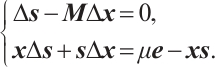 (2)
(2)
The system (2) gives the classical Newton search directions for  -LCP[24].
2 New Search Directions for  -LCP
-LCP
In preparation for the full-Newton step IPM, we first recall the AET technique for  -LCP. The AET technique for determining a new search direction for IPM involves transforming the centering equation
  of (1) into a new equation
  ,
,  .
.
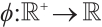
Now we give a search direction based on Darvay's method for  -LCP. We consider the power function
  which is monotonically increasing, continuously differentiable, and suppose that the invertible function
  exists. The system (1) can be written equivalently in the following form
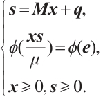 (3)
(3)
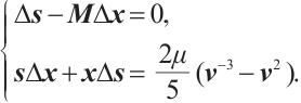
The natural way to define the search direction is to follow Newton's approach and linearize the system (3), which leads to the following system
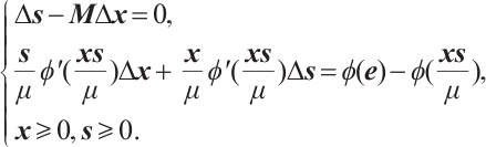 (4)
(4)
Since  is a
is a  matrix, this system uniquely defines the search directions
  and
and  . Then the new iterates are given by

By introducing the scaled search directions
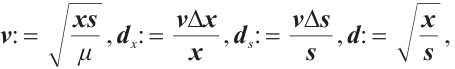 (5)
(5)
we can rewrite the system (4) as the following scaled Newton-system
 (6)
(6)
where 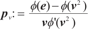 and
and 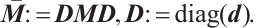 We observe that
  yields
  [7], which coincides with the classical Newton direction. Moreover, when
  equals
  and
and  , then
  corresponds to
  [16] and
  [25], respectively. Now let's take
  [22-23] based on Darvay's method, and we propose a new full-Newton IPM based on a novel appropriate search direction for
  -LCP. For the analysis of the algorithm, we define a norm-based proximity measure
  to the central path as follows:
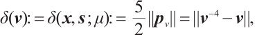 (7)
(7)
where
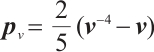 (8)
(8)
Clearly,

Let 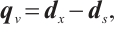 it is easy to obtain
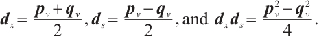
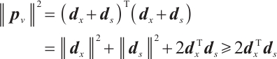
It is worthwhile to point out that the scaled search directions  and
and  are not orthogonal and
  is not always non-negative, which results in difficulties in the analysis of the algorithm for
  -LCP. In Section 3, some new techniques are used to solve this problem.
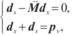
Moreover, by using (5), (6), (8), system (4) becomes
 (9)
(9)
Furthermore, we define the  -neighborhood of the central path as follows:
 (10)
(10)
where  is a threshold and
  .
.
Now we establish the full-Newton step IPM for  -LCP. Let's assume that the algorithm starts with a strictly feasible pair
  and
and 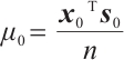 such that
 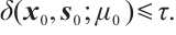 By using Newton's method, we can construct a new pair
  which is 'close' to
  . Then
  is reduced by the factor
  with
with  . This process is repeated until
  is small enough, i.e.,
  . Finally, an
  -approximate solution of (P) can be found through the following Algorithm 1.
Algorithm 1: A full-Newton step IPM for  -LCP based on a new AET technique -LCP based on a new AET technique |
|---|
|
Input: A threshold parameter  ; ;an accuracy parameter  ; ;barrier update parameter  ; ;a strictly feasible  and and  such that such that  begin  while  do dobegin 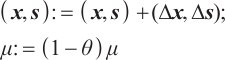 end end |
3 Analysis of the Algorithm
In this section, we first examine the feasibility of Algorithm 1 by establishing several technical lemmas. Subsequently, we provide a proof for the local quadratic convergence of a full-Newton step to the central path. Finally, we determine the polynomial iteration complexity of the algorithm.
3.1 Feasibility Analysis of the Algorithm
Lemma 1 The solution  of linear system (6) satisfies
 (11)
(11)
where 
Proof From Ref. [26], the solution  of linear system
  satisfies the following relations:
where  , therefore, by
we can deduce that
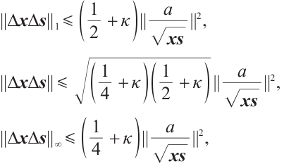
By 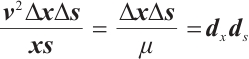 , we get the first three inequalities of (11). From (6), one get
and according to (7), we have  , hence, we obtain the last inequality.
Lemma 2 The full-Newton step is strictly feasible, i.e.  and
and  , provided that
  .
.
Proof Let  and
and  be a strictly feasible point for (P), then using (5), we get
 (12)
(12)
Due to (11) in Lemma 1 and (7) with  , it follows that
Now following from (12), for all  , we have
  if
if  . Here, we consider the function
  . It is easy to see that
  obtains a minimum at
  . Therefore, for all
  ,
,  , hence
 (13)
(13)
Thus  for
for  . Since
  and
and  , we obtain
  and
and  for all
  . Then, by continuity the vectors
  and
and  , i.e., the full-Newton step is strictly feasible. This completes the proof.
For convenience, we denote 
3.2 Convergence Analysis of the Algorithm
Lemma 3 If  , then
  .
.
Proof By setting  in (12), (13) and Lemma 1, one has
hence  . This completes the proof.
Next, we prove that the iteration of the proximity measure is locally quadratically convergent.
Lemma 4 Let  and
and  be a strictly feasible point for (P). Then
where  .
.
Furthermore, if  , then
  , which shows the quadratic convergence of the proximity measure.
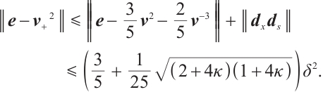
Proof We have 
Consider the function
Therefore, we can get

There is no difficulty to check that the function  is continuous, monotone decreasing and positive on
  . Hence,

Consequently
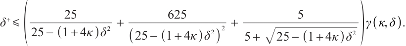
Next, setting  in (12), and from (8), we have
Recalling the proof of Lemma 4 in Ref. [23], we have
and together with (11), we obtain
This implies that
Letting  , by Lemma 3,
 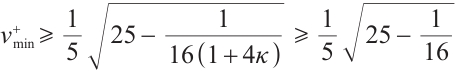 , we have
So we can get
which shows the quadratic convergence of the proximity measure. This completes the proof.
The next lemma shows the influence of a full-Newton step on the duality gap and gives an upper bound for it.
Lemma 5 If 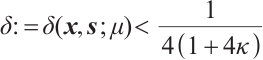 , then after a full-Newton step, the duality gap satisfies
 (14)
(14)
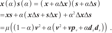
Proof Due to (5) and (7), we have
Then one gets
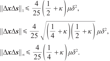
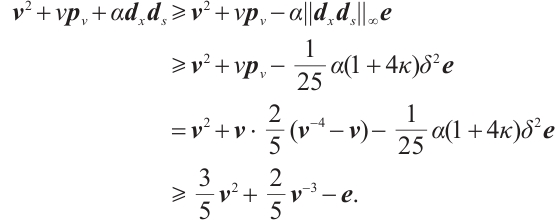
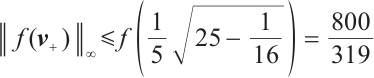
Since, after some reductions,  for all
  , see details in Lemma 4 of Ref. [23]. Then from the last inequality of (11) and (7), we get
  .
.
Using  , and
, and  , we may obtain
  This completes the proof.
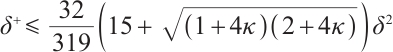
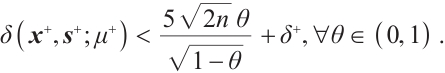
In the next theorem, we analyse the effect of a full-Newton step on the proximity measure by updating the parameter  by a factor
  .
.
Theorem 1 Let  and
and  , where
  , then
  .
.
Furthermore, if  and
and  , then we have
  .
.
Proof By 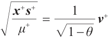 and
and 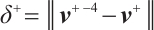 , one get
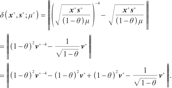
Using the triangular inequality, we get
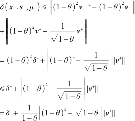
Given that  and
and  ,
,  , and also based on inequality (14) in Lemma 5, we have
  . Therefore, it can be concluded that
Using Lemma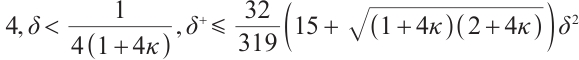 , we obtain the following inequality
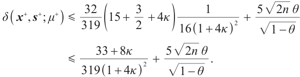
By 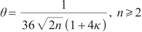 , one get
  . Moreover,
  , hence we have
This completes the proof of the theorem.
3.3 Complexity Analysis of the Algorithm
In the previous subsections, we have found that if at the start of an iteration, the iteration satisfies  with
with  , then after a full-Newton feasibility step, with
  as defined in Theorem 1, the iteration is strictly feasible and satisfies
  . Following this, we conclude this section by giving the iteration bound for Algorithm 1.
Lemma 6 Suppose that the pair  is strictly feasible,
  and
and  . Moreover, let
  be the point obtained after
  iterations. Then the inequality
  holds for
  .
.
Proof Due to  , then by (14) in Lemma 5,
Hence  holds, if
  , taking logarithms, one get
  .
.
Using inequality  , we obtain
  .
.
This proves the lemma.
Theorem 2 Let  and
and  , where
  . Then Algorithm 1 requires at most
  iterations that yield an
  -approximate solution of the
  -LCP in (P).
Proof Using defaults  and
and  , then the desired result follows directly from Lemma 6.
4 Numerical Results
In this section, we present some preliminary numerical results to assess the performance of the Algorithm 1. These results are compared with those obtained by the classical algorithm where the sum of the scaled directions  equals
  . The implementations are performed by using MATLAB 2014a on an Intel Core i5 processor (2.60 GHz) with 16 GB of RAM.We consider the following examples.
The first is a  -LCP with
  , and the last three are monotone LCPs, a significant subclass of
  -LCPs. For all experiments, we maintained a precision parameter of
  , and in Example 1, we set the parameters
  and
and  for Algorithm 1, with corresponding parameters
  ,
, for the classical algorithm[21]. However, in Example 2 and Example 3, we set the parameters
  and
and  for Algorithm 1, while
  ,
, for the classical algorithm[21]. The results of the three numerical experiments are summarized in Table 1.
Example 1 [27]
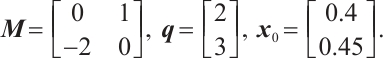
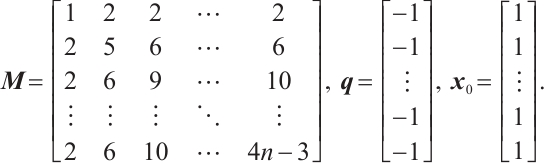
Example 2 [23]
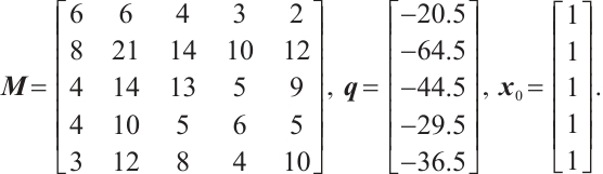
Example 3 [28]
In Table 1, "Iter" and "Time/s" denote the number of iterations and the CPU running time in seconds for these two algorithms, respectively. The result of Example 1 shows that Algorithm 1 has a better performance for  -LCP compared with the classical algorithm. And by Example 2 and Example 3, it shows that Algorithm 1 requires fewer iterations but has longer running times for
  -LCP. In particular, the number of iterations grows slowly as the problem size increases. This behaviour suggests that the proposed algorithm offers improved performance for large-scaled
  -LCPs.
To further verify the feasibility and efficiency of the proposed algorithm, we perform a series of random numerical experiments as follows. The results of the test are summarized in Table 2.
Example 4
Using MATLAB 2014a, we randomly generate a matrix  with row full rank and vectors
  , where
  are all one vectors. For this example, we take
  . Thus we obtain a corresponding test problem.
Table 2 shows the comparison between Algorithm 1 and the classical algorithm in terms of the number of iterations and CPU running time as the problem size  changes. From Table 2, in most cases, our algorithm uses fewer iterations and much less time to solve these problems, compared with the classical algorithm. It can be concluded that the algorithm proposed here is feasible and effective.
The numerical results of the  -LCP for different sizes
The numerical results for Example 4
5 Conclusion
In this study, we introduce and analyse a full-Newton step IPM for solving the  -LCP, based on a novel AET technique, which provides a new search direction for (P). The polynomial complexity of the algorithm is established, which coincides with the best-known iteration bound of currently feasible IPMs for
  -LCP. Elementary numerical results indicate the practical feasibility and efficiency of the proposed method. For future research, our efforts may focus on the design of infeasible IPM inspired by the AET technique discussed here, and on conducting more comprehensive numerical experiments for
  -LCP where
  is not equal to 0.
References
- Cottle R, Pang J S, Stone R E. The Linear Complementarity Problem[M]. Boston: Academic Press, 1992. [Google Scholar]
- Kojima M, Megiddo N, Noma T, Yoshise A. Progress in Mathematical Programming: A Primal-Dual Interior Point Algorithm for Linear Programming[M]. New York: Springer-Verlag, 1989. [Google Scholar]
- Wang G Q, Bai Y Q. A new primal-dual path-following interior-point algorithm for semidefinite optimization[J]. Journal of Mathematical Analysis and Applications, 2009, 353(1): 339-349. [Google Scholar]
- Wang G Q, Bai Y Q. A primal-dual interior-point algorithm for second-order cone optimization with full Nesterov-Todd step[J]. Applied Mathematics and Computation, 2009, 215(3): 1047-1061. [Google Scholar]
- Potra F A. A superlinearly convergent predictor-corrector method for degenerate LCP in a wide neighborhood of the central path with-iteration complexity[J]. Mathematical Programming, 2004, 100(2): 317-337. [Google Scholar]
- Kojima M, Megiddo N, Noma T, et al. A unified approach to interior point algorithms for linear complementarity problems: A summary[J]. Operations Research Letters, 1991, 10(5): 247-254. [Google Scholar]
- Illés T, Nagy M. A Mizuno-Todd-Ye type predictor-corrector algorithm for sufficient linear complementarity problems[J]. European Journal of Operational Research, 2007, 181(3): 1097-1111. [Google Scholar]
-
Wang G Q, Yu C J, Teo K L. A full-Newton step feasible interior-point algorithm for
 -linear complementarity problem[J]. Global Optimization, 2014, 59: 81-99.
[Google Scholar]
-linear complementarity problem[J]. Global Optimization, 2014, 59: 81-99.
[Google Scholar]
-
Zhang M W, Huang K, Li M M, et al. A new full-Newton step interior-point method for
 -LCP based on a positive-asymptotic kernel function[J]. Journal of Applied Mathematics and Computation, 2020, 64: 313-330.
[Google Scholar]
-LCP based on a positive-asymptotic kernel function[J]. Journal of Applied Mathematics and Computation, 2020, 64: 313-330.
[Google Scholar]
- Geng J, Zhang M W, Zhu D C. A full-Newton step feasible interior-point algorithm for the special weighted linear complementarity problems based on a kernel function[J]. Wuhan Univ J of Nat Sci, 2024, 29(1): 29-37. [Google Scholar]
- Geng J, Zhang M W, Pang J J. A full-Newton step feasible IPM for semidefinite optimization based on a kernel function with linear growth term[J]. Wuhan Univ J of Nat Sci, 2020, 25(6): 501-509. [Google Scholar]
- Yang Y G. A polynomial arc-search interior-point algorithm for linear programming[J]. Journal of Optimization Theory and Applications, 2013, 158(3): 859-873. [Google Scholar]
- Shahraki M S, Delavarkhalafi A. An arc-search predictor-corrector infeasible-interior-point algorithm for P(κ)-SCLCPs[J]. Numerical Algorithms, 2020, 83(4): 1555-1575. [Google Scholar]
- Yang Y G. Arc-Search Techniques for Interior-Point Methods[M]. Boca Raton: CRC press, 2020. [CrossRef] [Google Scholar]
- Yuan B B, Zhang M W, Huang Z G. A wide neighborhood arc-search interior-point algorithm for convex quadratic programming[J]. Wuhan Univ J of Nat Sci, 2017, 22(6): 465-471. [Google Scholar]
- Darvay Z. New interior-point algorithms in linear programming[J]. Advanced Modeling and Optimization, 2003, 5(1):51-92. [Google Scholar]
- Achache M. A new primal-dual path-following method for convex quadratic programming[J]. Computational & Applied Mathematics, 2006, 25(1): 97-110. [Google Scholar]
- Wang G Q, Lesaja G. Full Nesterov-Todd step feasible interior-point method for the Cartesian P*(κ)-SCLCP[J]. Optimization Methods and Software, 2013, 28(3): 600-618. [Google Scholar]
- Mansouri H, Pirhaji M. A polynomial interior-point algorithm for monotone linear complementarity problems[J]. Journal of Optimization Theory and Applications, 2013, 157(2): 451-461. [Google Scholar]
-
Asadi S, Mansouri H. Polynomial interior-point algorithm for
 horizontal linear complementarity problems[J]. Numerical Algorithms, 2013, 63: 385-398.
[Google Scholar]
horizontal linear complementarity problems[J]. Numerical Algorithms, 2013, 63: 385-398.
[Google Scholar]
-
Illés T, Rigó P R, Török R. Unified approach of interior-point algorithms for
 -LCP using a new class of algebraically equivalent transformations[J]. Optimization Theory and Applications, 2023, 202: 27-49.
[Google Scholar]
-LCP using a new class of algebraically equivalent transformations[J]. Optimization Theory and Applications, 2023, 202: 27-49.
[Google Scholar]
- Kheirfam B, Nasrollahi A. A full-Newton step interior-point method based on a class of specific algebra transformation[J]. Fundamenta Informaticae, 2018, 163(4): 325-337. [Google Scholar]
- Grimes W, Achache M. A path-following interior-point algorithm for monotone LCP based on a modified Newton search direction[J]. RAIRO-Operations Research, 2023, 57(3): 1059-1073. [Google Scholar]
- Darvay Z, Papp I M, Takács P R. Complexity analysis of a full-Newton step interior-point method for linear optimization[J]. Periodica Mathematica Hungarica, 2016, 73(1): 27-42. [Google Scholar]
- Darvay Z, Illés T, Majoros C. Interior-point algorithm for sufficient LCPs based on the technique of algebraically equivalent transformation[J]. Optimization Letters, 2021, 15(2): 357-376. [Google Scholar]
- Illés T, Nagy M, Terlaky T. A polynomial path-following interior point algorithm for general linear complementarity problems[J]. Journal of Global Optimization, 2010, 47(3): 329-342. [Google Scholar]
-
Lee Y H, Cho Y Y, Cho G M. Interior-point algorithms for
 -LCP based on a new class of kernel functions[J]. Journal of Global Optimization, 2014, 58(1): 137-149.
[Google Scholar]
-LCP based on a new class of kernel functions[J]. Journal of Global Optimization, 2014, 58(1): 137-149.
[Google Scholar]
- Harker Patrick T, Pang J S. A damped-Newton method for the linear complementarity problem[J]. Lectures in Applied Mathematics, 1990, 26: 265-284. [Google Scholar]
All Tables
Current usage metrics show cumulative count of Article Views (full-text article views including HTML views, PDF and ePub downloads, according to the available data) and Abstracts Views on Vision4Press platform.
Data correspond to usage on the plateform after 2015. The current usage metrics is available 48-96 hours after online publication and is updated daily on week days.
Initial download of the metrics may take a while.