| Issue |
Wuhan Univ. J. Nat. Sci.
Volume 30, Number 2, April 2025
|
|
|---|---|---|
| Page(s) | 169 - 183 | |
| DOI | https://doi.org/10.1051/wujns/2025302169 | |
| Published online | 16 May 2025 | |
Mathematics
CLC number: O212.1
Subgroup Analysis of a Single-Index Threshold Penalty Quantile Regression Model Based on Variable Selection
基于变量选择的单指标阈值惩罚分位数回归模型的亚组分析
1
School of Statistics and Mathematics, Zhongnan University of Economics and Law, Wuhan 430073, Hubei, China
2
Institute of Information Engineering, Sanming University, Sanming 365004, Fujian, China
3
Department of Biostatistics, School of Public Health, Fudan University, Shanghai 200032, China
Received:
28
June
2024
Abstract
In clinical research, subgroup analysis can help identify patient groups that respond better or worse to specific treatments, improve therapeutic effect and safety, and is of great significance in precision medicine. This article considers subgroup analysis methods for longitudinal data containing multiple covariates and biomarkers. We divide subgroups based on whether a linear combination of these biomarkers exceeds a predetermined threshold, and assess the heterogeneity of treatment effects across subgroups using the interaction between subgroups and exposure variables. Quantile regression is used to better characterize the global distribution of the response variable and sparsity penalties are imposed to achieve variable selection of covariates and biomarkers. The effectiveness of our proposed methodology for both variable selection and parameter estimation is verified through random simulations. Finally, we demonstrate the application of this method by analyzing data from the PA.3 trial, further illustrating the practicality of the method proposed in this paper.
摘要
在临床研究中,亚组分析可以帮助识别对特定治疗反应较好或较差的患者群体,提高治疗效果和安全性,在精准医疗中具有重要意义。为此,本文考虑了含有多个协变量和生物标志物的纵向数据下的亚组分析方法,并基于多个生物标志物的线性组合是否超过某一阈值来划分亚组,根据亚组与暴露变量间的交互作用来评估亚组间的异质效应。利用分位数回归方法更好地刻画响应变量的全局分布,并施加稀疏性惩罚实现协变量和生物标志物的变量选择。模拟研究验证了本文提出的估计方法在变量选择和参数估计方面的有效性,最后,将此方法应用到了PA.3试验的数据分析当中,进一步说明了本文方法的实用性。
Key words: longitudinal data / subgroup analysis / threshold model / quantile regression / variable selection
关键字 : 纵向数据 / 亚组分析 / 阈值模型 / 分位数回归 / 变量选择
Cite this article: QI Hui, XUE Yaxin. Subgroup Analysis of a Single-Index Threshold Penalty Quantile Regression Model Based on Variable Selection[J]. Wuhan Univ J of Nat Sci, 2025, 30(2): 169-183.
Biography: QI Hui, male, Associate professor, Ph. D. candidate, research direction: biostatistics, high dimensional statistics. E-mail: This email address is being protected from spambots. You need JavaScript enabled to view it.
Foundation item: Supported by the Natural Science Foundation of Fujian Province(2022J011177, 2024J01903) and the Key Project of Fujian Provincial Education Department(JZ230054)
© Wuhan University 2025
 This is an Open Access article distributed under the terms of the Creative Commons Attribution License (https://creativecommons.org/licenses/by/4.0), which permits unrestricted use, distribution, and reproduction in any medium, provided the original work is properly cited.
0 Introduction
Subgroups are usually defined based on biomarkers such as blood sugar, blood pressure, gene or protein expression levels, etc[1]. When evaluating the efficacy of new therapy on patients in clinical studies, these characteristic differences may lead to different responses of the same therapy to different patients[2]. Therefore, when physicians assess therapeutic effect, they should not only consider the average effect across the overall population, but also the heterogeneous effects within subgroups. Many methods for subgroup identification have proposed in research literature, such as method based on the tree structure[3], global model[4], clustering analysis[5], etc. In clinical practice, a straightforward and easily interpretable approach is often preferred, which involves dividing subgroups according to whether a single continuous biomarker exceeds a certain threshold. This is the threshold model we focus on.
However, in the threshold model described above, a single variable is used to classify subgroups, which can result in a limited representation of subgroup characteristics and may be compromised by the inappropriate choice of the threshold variable. Numerous studies suggest that subgroups may arise from the combined influence of multiple variables, for instance, Jiang et al[6] demonstrated that multiple single nucleotide polymorphisms (SNPs) can frequently alter the risk of developing specific diseases, whereas any single SNP alone lacks this capability; Fan et al[7] showed that a risk score defined as a function of multiple predictors is useful for identifying subgroups of AIDS patients who benefit more from treatment. Similarly, Vander Weele et al[8] discussed the importance of using multiple variables to identify optimal treatment subgroups. He et al[9] and Wei et al[10] extended this model to survival and longitudinal data, respectively. While they utilized penalization methods to identify significant biomarkers, they did not perform variable selection for the included covariates.
Moreover, the majority of current studies on threshold model primarily focus on traditional mean regression. However, sometimes we place greater emphasis on sample data at other quantiles, for example, we prefer to conduct heterogeneity analysis on patients with worse condition and provide targeted medical solutions. Consequently, we consider introducing quantile regression to analyze the threshold model. The threshold quantile regression was initially introduced by Cai et al[11] and applied to quantile self-exciting threshold autoregressive time series models. Galvao et al[12] studied the threshold quantile autoregressive processes. Furthermore, Lee et al[13] developed the general tests for threshold effects in regression models, Su and Xu[14] presented a systematic estimation and inference procedure for threshold quantile regression. On this basis, Zhang et al[15] proposed a more general single-index threshold quantile regression model. However, there is no existing literature that addresses the variable selection for covariates and biomarkers in single-index threshold quantile regression.
In practical applications, incorporating excessive number of biomarkers for subgroup division may diminish the interpretability of the subgroups, and including excessive number of covariates may also introduce multicollinearity. Consequently, we prefer to select the variables most pertinent to the response from the model's explanatory variables. Common variable selection methods include those based on penalties. This method, initially proposed by Tibshirani in 1996[16], is known as Lasso estimation, which uses an L1 norm penalty. Subsequent researches include: Fused Lasso penalty[17], Adaptive Lasso[18], Graphical Lasso[19] and so on. Furthermore, as Lasso compresses all coefficients equally, the resulting estimator is often biased. To this end, Fan et al[20] introduced the smoothly clipped absolute deviation (SCAD) penalty and proved that the estimation result satisfied the oracle property.
Our paper extends the single-index threshold quantile regression[15] to longitudinal data and introduces the SCAD penalty for variable selection of covariates and biomarkers. To this end, we propose an efficiency algorithm similar to that proposed by Zhang et al[21], which transforms the problem of estimating the covariate regression coefficients and threshold parameters into a penalized linear quantile regression. Furthermore, we obtain a degraded linear quantile regression through pseudo observations. In addition, the penalty for covariates and biomarkers should be performed separately. We combine the two-step grid search algorithm[22] to select the compression parameters that minimize the Bayesian information criterion (BIC), and then substitute the pre-selected compression parameters into the iterative algorithm for parameter estimation. Finally, random simulations and example analysis illustrate the practicality of our method.
1 Models and Estimation
We assume that  is the response variable of the i-th individual at the j-th observation,
 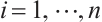 ,
,  , total observations
  ,
,  is the covariates with dimension of
  , where
  ,
,  is a subset of
  , and xi=
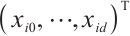 is the baseline biomarker including the intercept term. We consider the following single-index threshold quantile regression with

The regression coefficients  characterize the baseline effect of
  at the
  -quantile of
  , and the regression coefficients
  describe the heterogeneity of
  within the subgroup, the threshold coefficients
  determine the subgroup based on whether the linear combination
  exceeds 0. We consider time-invariant biomarkers to prevent time-varying biomarkers from dividing repeated observations of the same sample into different subgroups due to the influence of treatment. In addition, the error terms
  and
and  are typically assumed to be independent for any
  stemming from the index set
  , but correlated within
  for any fixed
  . Assume
For the recognizability of  , reference Zhang et al[15] and Horowitz[23], assuming that at least one threshold variable has a nonzero coefficient, and the corresponding probability distribution is absolutely continuous with respect to the Lebesgue measure conditional on the other threshold variables. The variables in
  can be rearranged so that
  meets this condition, then the model can be rewritten as:

where  ,
, with
with  and
and  corresponding to the coefficients of
  and
and  , respectively. If
  is positive, the normalization without altering the coefficients of
  and
and  . If
. If  is negative, we should redefined
  and
and  to ensure the consistency of the model[15]. Moreover, for the convenience of expression, we remove
  in the parameters below.
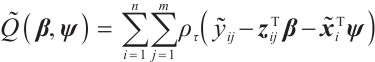
In order to estimate all parameters  , a computationally efficient method is to ignore the possible correlation between repeated observations within the longitudinal data, that is, to minimize the following objective function under the independence framework:
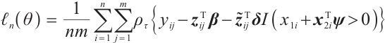
where  is the quantile loss function. In order to address the challenge of discontinuity in the objective function, similar to Seo and Linton[24], we employ an integrated kernel function to smooth this characteristic function, for example, the cumulative distribution function of the standard normal distribution
  , then we can derive the smoothing objective function as following:
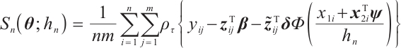
In refer to Zhang et al[15], this article selects the bandwidth 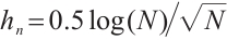 .
.
Furthermore, it is hoped to select important covariates  and threshold variables
  . In practice, a few exposure variables of interest are included in
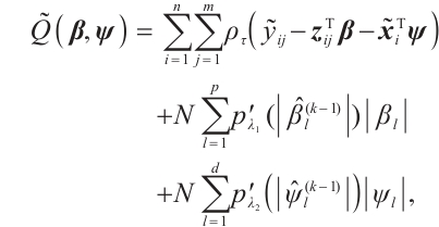
  , such as treatment group indices or drug doses, thus variable selection for interaction terms is not considered. Consequently, the objective function, which includes corresponding penalty terms, is formulated as:
where  is the penalty function, and
  and
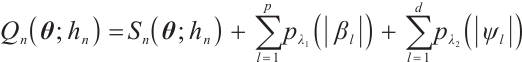
and  are the shrinkage adjustment parameters that control the partial linear regression parameters and threshold parameters, respectively. We consider the following non-convex SCAD penalty function:
when  , and
, and  . SCAD penalty approaches the optimal Bayesian risk[20], therefore, the nuisance parameters involved in the model only are
  and
and  .
.
Since the objective function  is non-convex and not differentiable everywhere, we use the local linear approximation algorithm of Zou and Li[25] to transform the non-convex SCAD penalty into a convex approximation form. Specifically,


Moreover, even if we employ a profile estimation similar to Zhang et al[15] to estimate the slope  and threshold parameters
  separately, the objective function is still non-convex with respect to
  with fixing
  . Owing to the slow computation speed of genetic algorithms and the sensitivity of the Nelder-Mead method to initial values, therefore, we employ the first-order Taylor linear approximation to
  ,
,
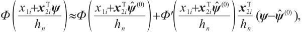
where  indicates the probability density function of the standard normal distribution. Accordingly, with initial estimation for
  and
and  , we can derive a new objective function
  with respect to
  and
and  :
:
and
Now, the estimation of  and
and  is essentially a penalized linear quantile regression problem, specific iterative algorithm is as follows:
Step 0 Initialize  .
.
Step 1 Given 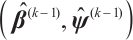 , we have:
Step 2 Given  , the estimation
  is derived by minimizing the following objective function:
and
set 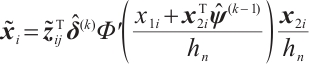 , repeat step 1 and step 2 until the L2 norm of adjacent estimation for all parameters are less than the tolerance error.
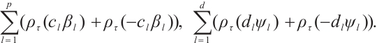
Finally, according to the facts 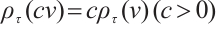 and
and 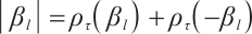 , set
, set 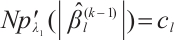 , and
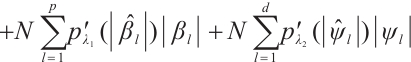
, and 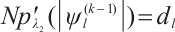 , then, we rewrite the first and second penalty terms as follows:
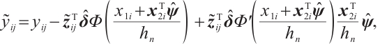
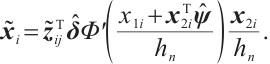
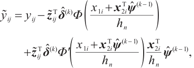
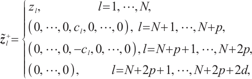
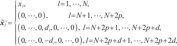
Furthermore, we construct the "unpenalized" linear quantile regression through incorporating additional pseudo observations. The augmented form of the defining variables is as follows:
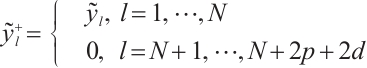
then the objective function in Step 2 degenerates into linear quantile regression: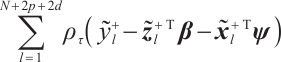 ,and proceed with solving it.
In practice, BIC is frequently employed in variable selection problems for tuning parameter selection,
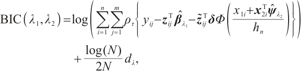
 represents the total count of non-zero coefficients in both the slope and threshold components, while
  denotes the total number of observations. Following Ruppert and Carroll[22], we employ a two-step grid search algorithm to derive the optimal tuning parameters
  .
.
2 Simulation
In order to assess the performance of our proposed estimation in finite samples, we consider the following data generation model:

covariates 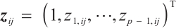 , and
, and  ,
,  , the remaining covariates
  are independent and conform to uniform distribution
  ; interaction variable
  , threshold variables
  , component
  within
  , the remaining covariates
  are independent and conform to uniform distribution
  too; setting
  ,
,  , and
, and  . However, in our data generation model, the true value of
  varies with the quantile. The random error term
  , where
  ensures
  , we take into account two error distributions:
Case 1 The random error vector conforms to multivariate normal distribution, that is, 
 , and the covariance matrix
  follows
  -1 correlation structure with correlation coefficient
  , where the partial coefficients of the model are set to

Case 2 The random error vector conforms to multivariate  distribution, that is,
 , and the covariance matrix shares the same structure, where
 ,
, 
 is the
  quantile of the
  distribution with degrees of freedom (df) 3.
We will assess the performance of our estimation across varying numbers of parameters  or
or  or different quantiles
  , each random experiment yields
 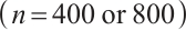 samples, with each sample being observed
  times, and the simulation is repeated 500 times. We assess the model's performance using four criterias: 1) True Negative (TN): This represents the average number of zero parameters that are correctly classified as zero by the model. A higher TN indicates better model performance; 2) False Negative (FN): The average number of non-zero parameters erroneously classify as zero. A lower FN indicates better model performance; 3) Correct (%): This represents the percentage of accurate true models with non-zero parameters that are correctly identified. The closer this percentage is to 100, the more accurate the model estimation effect is; 4) MSE: It represents the mean square error of the parameter estimation, smaller MSE indicates that the estimated value
  is closer to the true value
  , and the better estimation effect of the model. By comparing the mean square error O.MSE of the oracle estimator with the mean square error P.MSE of our method, the P.MSE is closer to O.MSE means the better estimation effect of our approach.
Tables 1 and 2 present the variable selection outcomes of the single-index threshold quantile regression when the error terms follow a multivariate normal distribution or a multivariate T(3) distribution, respectively. In an ideal scenario, the component of TN for the linear segment is  , and for the threshold segment it is
  . The oracle TN in scenario
  and scenario
  is 15 or 35, respectively. In all settings, our method can compress the true zero coefficients to zero and correctly identify all relevant covariates (FN=0), with P.MSE and the O.MSE is very close, which indicate that the model estimation is very effective.
Tables 3 and 4 show the estimators of the identified nonzero parameters by our method when the error terms follow a multivariate normal distribution or a multivariate T(3) distribution, respectively. The Biases for all nonzero parameters remain minimal across various parameter counts  or
or  or quantiles
  , and all metrics: Biases, SDs, and RMSEs decrease as the sample size increases.
We further conduct sensitivity comparisons for two bandwidths  and
and  under
under  ,
,  , while keeping the remaining settings as the same as before. The RMSEs of the proposed estimators in Fig. 1 show that these two bandwidths do not exert significant effects on the performance of the proposed method
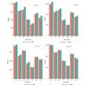 |
Fig. 1 The sensitivity diagram of parameter estimation under the bandwidth rates  and and  with with  and and 
|
Variable selection in the case where  and
and  follows an
  -1 structure
Variable selection in the case where  and
and  follows an
  -1 structure
Estimation results of parameters in the case where  and
and  follows an
  -1 structure
Estimation results of parameters in the case where  and
and  follows an
  -1 structure
3 Real Data Analysis
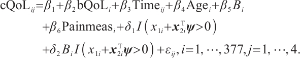
We apply the proposed method to analyze the PA.3 trial dataset conducted by the Canadian Cancer Group. In this trial, patients with locally advanced or metastatic pancreatic cancer were randomly assigned to the erlotinib plus gemcitabine group or the gemcitabine monotherapy group. In the primary analysis, the survival rate of the erlotinib plus gemcitabine group was significantly improved compared with the gemcitabine monotherapy group[26]. Shultz et al[27] found that when each biomarker was evaluated individually, none of them was significantly associated with erlotinib. However, He et al[9] selected CA19-9 and AXL from 47 biomarkers to define the treatment-sensitive subgroup, and found that the erlotinib plus gemcitabine could prolong patient's survival time compared with gemcitabine monotherapy. Similarly, Wei et al[10] selected CA19-9 and AXL from 6 biomarkers to define a treatment-sensitive subgroup and found that erlotinib plus gemcitabine improved patient's quality of life (QoL) scores compared with gemcitabine monotherapy. However, these studies only focused on selecting biomarkers for defining subgroups, not covariates. Moreover, none of these studies investigated whether distinct subgroup effects exist in patients across various QoL levels. Therefore, we use our method to select relevant covariates and biomarkers, and assess the differential therapeutic effect of erlotinib in subgroups defined by linear combinations of these biomarkers, as well as the differences in effects at different quantile levels of the outcomes.
A total of 377 patients were included in the analysis, of whom 196 received erlotinib treatment, and their quality of life was assessed using the global QoL score. For each patient in the trial, QoL scores were recorded at the baseline, as well as 4, 8, 12, and 16 weeks following the treatment. We focus on the changes in patient's QoL scores relative to the baseline (cQoL), and missing values have imputed using multiple imputation. The Q-Q plot of the imputed variable  and the Shapiro-Wilk normality test indicate that the data do not conform to a normal distribution. The calculated skewness is 0.139 3, indicating a right skewed distribution, so that quantile regression is considered to be more suitable than the mean regression. The covariates included in the analysis are: baseline QoL score (bQoL), time point (Time), baseline age (Age), treatment index B (if the patient received erlotinib plus gemcitabine, B = 1; if the patient received gemcitabine alone, B=0), and pain level (Painmeas). The twelve biomarkers included in the analysis include proteins with lower overall survival and baseline expression levels associated with metastatic diseases, specifically: AXL: AXL receptor tyrosine kinase; CA 19-9: Carbohydrate antigen 19-9; IL8: Interleukin-8; CEA: Carcinoembryonic antigen; MUC-1: Mucin 1, cell surface associate; PDGFRA: Platelet-derived growth factor receptor; EGFR: Epidermal growth factor receptor; PDK1: Pyruvate dehydrogenase kinase 1; BMP-2: Bone morphogenetic protein 2; HER2: Erb-b2 receptor tyrosine kinase 2; PF4: Platelet factor 4; GAS6: Growth arrest-specific protein 6. We standardize the 12 biomarkers and impute missing values using the median.
It is worth noting that our model requires the development of significant biomarker and assumes its coefficient to be nonzero. With prior knowledge, we should primarily consider results from expert opinions or existing literature. In terms of analyzing the PA.3 dataset, existing literature has selected CA19-9 and AXL as significant biomarkers in mean regression[10] and Cox regression[9] analysis based on threshold models for
  . Hence, we may consider utilizing CA19-9 or AXL as significant threshold variable for defining subgroups, with one designate as
  and the rest store in
  , we can also compare the differences in subgroup analysis when different biomarker is designated as
  . We construct the following single-index threshold quantile regression to fit the data:
Set  ,
, ,
,  ,
,  -
- ,
,  -
- ,
,
 -
- -
-

 represents the part of
  minus
minus  , assuming that the error term satisfies
  .
.
In order to conduct subgroup analysis of outcome variables at different levels as comprehensively as possible, we consider 7 quantile levels 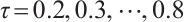 , and the same two-step grid search method as in the simulation study is used to select the tuning parameters
  and
and  . Table 5 presents the point estimator, bootstrap standard error (BS-SE), 95% confidence interval (95%-CI), and p-value of each parameter obtained at the above quantile levels with fixing
  .
.
From Table 5, it can be seen that in terms of variable selection, our method sets the coefficients for observation time (Time) and treatment index variable (B) to 0 across all quantiles ranging from 0.2 to 0.8, additionally, it sets the coefficients for age (Age) to 0 at quantiles 0.4 to 0.8, while the effect at quantiles 0.2 to 0.3 have not statistically significant. Thus, we conclude that the effects of observation time (Time) and age (Age) on patient's QoL scores are not significant. However, the selection of treatment effect (B) as an unrelated variable may be due to the masking of the interaction effect between treatment and subgroups, resulting in an insignificant effect, which requires further confirmation in stratified analysis. In addition, CA19-9 is selected as an important biomarker at all quantiles, and the coefficients of the remaining 10 biomarkers are compressed to 0. The biomarkers we selected are consistent with the results of He et al[9] and Wei et al[10].
In terms of subgroup analysis, within the mid or low percentiles (0.2-0.6), the p-value of the interaction coefficient  between treatment and subgroup is less than 0.05, this demonstrates a significant difference in therapeutic effect between the two subgroups at the 0.05 significance level. However, within the high percentile range (0.7-0.8), the corresponding p-value is met with
  , this demonstrates that the difference in therapeutic effect between the two subgroups is not significant at the 0.05 significance level, the possible reason is that there is no treatment sensitive subgroup, and further exploration is required through stratified analysis.
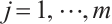
Next, we define the biomarker positive subgroup and the biomarker negative subgroup according to linear combination of fixing biomarker AXL, intercept and selected biomarker CA19-9, corresponding coefficients  as shown in Table 5. Linear quantile regression has conducted on all covariates separately for the samples in two subgroups, the estimated therapeutic effect and their 95% confidence intervals at different quantiles present in Fig. 2, and the confidence intervals are derived from rank tests. Figure 2 reveals that there is significant heterogeneity in therapeutic effect between the two subgroups. Specifically, at all quantiles, within the biomarker positive subgroup, the therapeutic effect are all significant positive values, and the 95% confidence intervals mostly fall above the zero line, which indicate that erlotinib has a positive impact on improving QoL scores. Therefore, we believe that at fixed
  , the identified biomarker positive subgroup is the treatment sensitive subgroup, in which patients receiving treatment of erlotinib plus gemcitabine have significantly improved quality of life scores compared to treatment with gemcitabine alone. However, within the biomarker negative subgroup, the 95% confidence interval for therapeutic effect remains zero, which indicates that the results are not significant. Therefore, we believe that in this subgroup, patients do not benefit more from erlotinib plus gemcitabine treatment compared to treatment with gemcitabine alone.
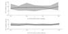 |
Fig. 2 The 95% confidence intervals of therapeutic effect when fixing 
|
Moreover, Table 6 presents the same four estimators at the corresponding quantile level with fixing  -9. As can be seen from Table 6, the corresponding main results of variable selection and subgroup analysis are similar to those in Table 5 with fixing
  .
.
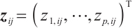
Similarly, we also define the biomarker positive subgroup and the biomarker negative subgroup according to linear combination of fixing biomarker CA19-9. The corresponding estimated therapeutic effect and their 95% confidence intervals at different quantiles present in Fig. 3. Figure 3 shows that there is still significant heterogeneity in the therapeutic effect between the two subgroups. But unlike in the case of fixing  , when
  -9 is fixed, the treatment sensitive subgroup with significant therapeutic effect is the identified biomarker negative subgroup, patients in this subgroup who receive treatment with erlotinib plus gemcitabine will significantly improve their overall quality of life score, however, within the biomarker positive subgroup, patients did not benefit more from the combination therapy of erlotinib and gemcitabine. This indicates that the 0-1 values of the subgroup index variables have reversed in both scenarios, that is, the interaction coefficient
  between treatment and subgroups is negative when
 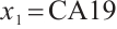 -9, and positive when
  . It also explains why the coefficient
  of the treatment term is selected as a significant correlation variable when
  -9, while it is compressed to 0 when
  .
.
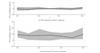 |
Fig. 3 The 95% confidence intervals of therapeutic effect when fixing -9 -9
|
In summary, combining the results of subgroup analysis for setting  and
and  -9, we can see that our method can identify treatment sensitive subgroups. In this subgroup, patients receiving treatment of erlotinib plus gemcitabine are more beneficial in improving their QoL score compared with using gemcitabine alone, and erlotinib is effective for patients with different QoL levels.
Finally, when fixing  or
or  -9 separately, we also want to compare whether the defined subgroups are consistent. We draw Fig. 4 to visualize the overlap of the subgroups divided in both cases, when fixing
  , the treatment sensitive subgroup corresponding to the biomarker positive subgroup is defined as group 1; the treatment insensitive subgroup corresponding to the biomarker negative subgroup is defined as group 2. Conversely, when fixing
 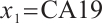 -9, the treatment sensitive subgroup corresponding to the biomarker negative subgroup is defined as group 1; the treatment insensitive subgroup corresponding to the biomarker positive subgroup is defined as group 2. Figure 4 shows the intersection and union of group 1 and group 2 in two different scenarios, the orange bars corresponding to 11 indicate that they are all assigned to group 1 in both scenarios, the blue bars corresponding to 22 signify that they are all assigned to group 2, 12 and 21 represent the number of individuals assigned to distinct subgroups in each scenario, with no intersection, and are uniformly displayed with gray bars.
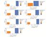 |
Fig. 4 Schematic diagram of subgroup overlap for two different settings |
In order to clearly display the proportion of patients divided into different subgroups in both scenarios, we set the highest count point of each subgraph to 100 and compare the height of the orange and gray bars. It can be found that the overlap of the treatment sensitive subgroups identified in both scenarios is very high, which indicates that the application of our method for subgroup identification has good robustness in the selection of  .
.
Estimation results of parameters when fixing 
Estimation results of parameters when fixing  -9
-9
4 Conclusion
This article considers a single-index threshold quantile regression for subgroup analysis, and selects covariates and biomarkers for defining subgroups, an efficient algorithm is proposed to smooth and locally linearly approximate the subgroup index function and non-convex penalty, respectively. Based on pseudo observations, the corresponding estimation problem degenerates into linear quantile regression, and all unknown parameters are iteratively solved through a two-step estimation process. Numerical simulations demonstrate that the proposed algorithm performs well with a moderate number of variables. Analysis of real data from the PA.3 trial shows that it can distinguish patient between treatment sensitive and treatment insensitive subgroups.
However, our model only considers the case of one threshold, so patient can only be divided into two subgroups. Furthermore, multiple thresholds can be introduced to divide subjects into multiple subgroups with different covariate effects, for related studies, please refer to Li et al[28-29]. In addition, the recognizability constraint in our model requires specifying a threshold variable  with non-zero coefficient. In practical applications, this variable can be determined through professional knowledge. However, when prior knowledge is not available, it may be achieved by extending the score type specification test method designed by Zhang et al[30] for selecting the non-zero threshold variables. In addition, considering the internal correlation of longitudinal data and conducting variable selection and parameter estimation under certain condition
  is our future research direction.
References
- Alosh M, Huque M F, Bretz F, et al. Tutorial on statistical considerations on subgroup analysis in confirmatory clinical trials[J]. Statistics in Medicine, 2017, 36(8): 1334-1360. [Google Scholar]
- Sachdev J C, Sandoval A C, Jahanzeb M. Update on precision medicine in breast cancer[J]. Cancer Treatment and Research, 2019, 178: 45-80. [Google Scholar]
- Su X, Tsai C L, Wang H, et al. Subgroup analysis via recursive partitioning[J]. Journal of Machine Learning Research, 2009, 10(2): 141-158. [Google Scholar]
- Lipkovich I, Dmitrienko A, Denne J, et al. Subgroup identification based on differential effect search: A recursive partitioning method for establishing response to treatment in patient subpopulations[J]. Statistics in Medicine, 2011, 30(21): 2601-2621. [Google Scholar]
- Zhang Z H, Seibold H, Vettore M V, et al. Subgroup identification in clinical trials: An overview of available methods and their implementations with R[J]. Annals of Translational Medicine, 2018, 6(7): 122. [Google Scholar]
- Jiang Z Y, Du C G, Jablensky A, et al. Analysis of schizophrenia data using a nonlinear threshold index logistic model[J]. PLoS One, 2014, 9(10): e109454. [Google Scholar]
- Fan A L, Song R, Lu W B. Change-plane analysis for subgroup detection and sample size calculation[J]. Journal of the American Statistical Association, 2017, 112(518): 769-778. [Google Scholar]
- Vander Weele T J, Luedtke A R, Vander Laan M J, et al. Selecting optimal subgroups for treatment using many covariates[J]. Epidemiology, 2019, 30(3): 334-341. [Google Scholar]
- He Y, Lin H Z, Tu D S. A single-index threshold Cox proportional hazard model for identifying a treatment-sensitive subset based on multiple biomarkers[J]. Statistics in Medicine, 2018, 37(23): 3267-3279. [Google Scholar]
- Wei K C, Zhu H C, Qin G Y, et al. Multiply robust subgroup analysis based on a single-index threshold linear marginal model for longitudinal data with dropouts[J]. Statistics in Medicine, 2022, 41(15): 2822-2839. [Google Scholar]
- Cai Y Z, Stander J. Quantile self-exciting threshold autoregressive time series models[J]. Journal of Time Series Analysis, 2008, 29(1): 186-202. [Google Scholar]
- Galvao Jr A F, Montes‐Rojas G, Olmo J. Threshold quantile autoregressive models[J]. Journal of Time Series Analysis, 2011, 32(3): 253-267. [Google Scholar]
- Lee S, Seo M H, Shin Y. Testing for threshold effects in regression models[J]. Journal of the American Statistical Association, 2011, 106(493): 220-231. [Google Scholar]
- Su L J, Xu P. Common threshold in quantile regressions with an application to pricing for reputation[J]. Econometric Reviews, 2019, 38(4): 417-450. [Google Scholar]
- Zhang Y Y, Wang H J, Zhu Z Y. Single-index thresholding in quantile regression[J]. Journal of the American Statistical Association, 2022, 117(540): 2222-2237. [Google Scholar]
- Tibshirani R. Regression shrinkage and selection via the lasso[J]. Journal of the Royal Statistical Society Series B: Statistical Methodology, 1996, 58(1): 267-288. [CrossRef] [Google Scholar]
- Tibshirani R, Saunders M, Rosset S, et al. Sparsity and smoothness via the fused lasso[J]. Journal of the Royal Statistical Society Series B: Statistical Methodology, 2005, 67(1): 91-108. [Google Scholar]
- Zou H. The adaptive lasso and its oracle properties[J]. Journal of the American Statistical Association, 2006, 101(476): 1418-1429. [CrossRef] [Google Scholar]
- Friedman J, Hastie T, Tibshirani R. Sparse inverse covariance estimation with the graphical lasso[J]. Biostatistics, 2008, 9(3): 432-441. [CrossRef] [PubMed] [Google Scholar]
- Fan J Q, Li R Z. Variable selection via nonconcave penalized likelihood and its oracle properties[J]. Journal of the American Statistical Association, 2001, 96(456): 1348-1360. [CrossRef] [Google Scholar]
- Zhang Y, Lian H, Yu Y. Ultra-high dimensional single-index quantile regression[J]. Journal of Machine Learning Research, 2020, 21(224): 1-25. [Google Scholar]
- Ruppert D, Carroll R J. Theory & methods: Spatially-adaptive penalties for spline fitting[J]. Australian & New Zealand Journal of Statistics, 2000, 42(2): 205-223. [Google Scholar]
- Horowitz J L. A smoothed maximum score estimator for the binary response model[J]. Econometrica, 1992, 60(3): 505. [Google Scholar]
- Seo M H, Linton O. A smoothed least squares estimator for threshold regression models[J]. Journal of Econometrics, 2007, 141(2): 704-735. [Google Scholar]
- Zou H, Li R Z. One-step sparse estimates in nonconcave penalized likelihood models[J]. Annals of Statistics, 2008, 36(4): 1509-1533. [Google Scholar]
- Moore M J, Goldstein D, Hamm J, et al. Erlotinib plus gemcitabine compared with gemcitabine alone in patients with advanced pancreatic cancer: A phase III trial of the National Cancer Institute of Canada Clinical Trials Group[J]. Journal of Clinical Oncology, 2007, 25(15): 1960-1966. [Google Scholar]
- Shultz D B, Pai J, Chiu W, et al. A novel biomarker panel examining response to gemcitabine with or without erlotinib for pancreatic cancer therapy in NCIC clinical trials group PA.3[J]. PLoS One, 2016, 11(1): e0147995. [Google Scholar]
- Li J L, Jin B S. Multi-threshold accelerated failure time model[J]. The Annals of Statistics, 2018, 46(6A): 2657-2682. [Google Scholar]
- Li J L, Li Y G, Jin B S, et al. Multithreshold change plane model: Estimation theory and applications in subgroup identification[J]. Statistics in Medicine, 2021, 40(15): 3440-3459. [Google Scholar]
- Zhang L W, Wang H J, Zhu Z Y. Testing for change points due to a covariate threshold in quantile regression[J]. Statistica Sinica, 2014, 24(4): 1859-1877. [Google Scholar]
All Tables
All Figures
|
Fig. 1 The sensitivity diagram of parameter estimation under the bandwidth rates and with and
|
| In the text | |
|
Fig. 2 The 95% confidence intervals of therapeutic effect when fixing
|
| In the text | |
|
Fig. 3 The 95% confidence intervals of therapeutic effect when fixing-9
|
| In the text | |
|
Fig. 4 Schematic diagram of subgroup overlap for two different settings |
| In the text | |
Current usage metrics show cumulative count of Article Views (full-text article views including HTML views, PDF and ePub downloads, according to the available data) and Abstracts Views on Vision4Press platform.
Data correspond to usage on the plateform after 2015. The current usage metrics is available 48-96 hours after online publication and is updated daily on week days.
Initial download of the metrics may take a while.