| Issue |
Wuhan Univ. J. Nat. Sci.
Volume 31, Number 2, April 2026
|
|
|---|---|---|
| Page(s) | 101 - 111 | |
| DOI | https://doi.org/10.1051/wujns/2026312101 | |
| Published online | 13 May 2026 | |
Aquatic Ecology and Water Environment Safety
CLC number: O175.25
Qualitative Analysis and Numerical Simulation of a Predator-Prey Model for Invertebrate Predators in Aquatic Population Ecosystem
水生种群生态系统中具有无脊椎捕食者的捕食食饵模型定性分析与数值模拟
School of Mathematics and Information Science, Baoji University of Arts and Sciences, Baoji 721013, Shaanxi, China
(宝鸡文理学院 数学与信息科学学院, 陕西 宝鸡721013)
† Corresponding author. E-mail: This email address is being protected from spambots. You need JavaScript enabled to view it.
Received:
20
April
2025
Abstract
The predation mechanism of invertebrates (e.g., Tortanus dextrilobatus) on plankton in aquatic population ecosystem is a significant research topic. In this paper, the interaction between invertebrates and plankton is simulated by a modified Leslie-Gower predator-prey model. Using the theory of reaction-diffusion equations, a priori estimate, existence, uniqueness and stability conditions of the positive steady state solution are established. Furthermore, numerical simulations are conducted to quantitatively analyze the dynamical behavior. The research shows that as long as the Allee effect constant satisfies the appropriate relationship and the growth rates of predator and prey are appropriately large, the predator and prey can not only coexist, but also the coexistence mode is unique and stable under low predation-rate. In addition, the numerical simulations show that the coexistence may be stable under high predation-rate. Meanwhile, with the increase of predation rate, the population density of predators will decrease.
摘要
无脊椎动物(例如溞溏水蚤)对水生种群生态系统中浮游生物的捕食机制是一个重要的研究课题。本文采用改进的Leslie-Gower捕食-食饵模型模拟了无脊椎动物和浮游生物之间的相互作用。利用反应扩散方程理论,建立了正稳态解的先验估计、存在性、惟一性和稳定性条件。此外,利用数值模拟定量分析了模型动力学行为。研究表明,只要Allee效应常数满足适当的关系、捕食者和食饵的生长速度适当大,捕食者和食饵不仅可以共存,而且在低捕食率下共存模式是惟一且稳定的。此外,数值模拟表明,在高捕食率下,也可能共存。同时,随着捕食率的增加,捕食者的种群密度会减小。
Key words: predator-prey model / aquatic population ecosystem / Allee effect / Ivlev functional response / positive steady-state solutions / numerical simulation
关键字 : 捕食-食饵模型 / 水生种群生态系统 / Allee效应 / Ivlev型功能反应函数 / 正稳态解 / 数值模拟
Cite this article:WANG Lijuan, JIANG Hongling, HE Jinchan, et al. Qualitative Analysis and Numerical Simulation of a Predator-Prey Model for Invertebrate Predators in Aquatic Population Ecosystem[J]. Wuhan Univ J of Nat Sci, 2026, 31(2): 101-111.
Biography: WANG Lijuan, female, Master candidate, research direction: partial differential equations. E-mail:This email address is being protected from spambots. You need JavaScript enabled to view it.
Foundation item: Supported by the National Natural Science Foundation of China (11961030) , the Natural Science Foundation of Shaanxi Province (2022JM-034)
© Wuhan University 2026
 This is an Open Access article distributed under the terms of the Creative Commons Attribution License (https://creativecommons.org/licenses/by/4.0), which permits unrestricted use, distribution, and reproduction in any medium, provided the original work is properly cited.
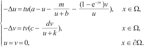
0 Introduction
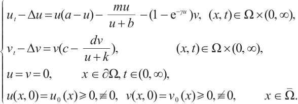
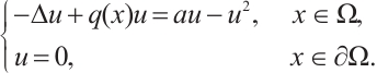
Let's start with the following predator-prey model
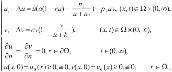 (1)
(1)
where  is a bounded domain with smooth boundary
  . In Ref. [1], the authors studied the predator-prey model (1) and gave the conditions for the steady-state bifurcation and Hopf bifurcation from the unique positive constant solution. The
  used here named additive Allee effect, where
  and
and  are constants of Allee effect which describing the strength of Allee effect, refers to that the low density populations may have difficulties in finding mates, promoting reproduction, predation, environmental regulation and inbreeding, which may lead to population extinction. Therefore, it is significant to study the mechanism of Allee effect to avoid population extinction in low density population. Some classic studies on the impact of Allee effect on predation models can be found in Refs. [2-5]. The background and parameter meanings of this model can be found in Ref. [1] and we omit here.
It is well known that the predator-prey functional response is an important factor in predator-prey models, which profoundly affects the dynamics of predator-prey models[6-7]. The functional response  in (1) is linear function and is unbounded. This deficiency reminds us that we can use the following Ivlev function, which can be written as
 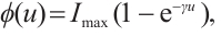 where
where  is the population density of prey,
  and
and  are positive constants which represent the predation rate of the predator and the maximum capture rate, respectively. It is clear that the
  is bounded and satisfies
A recent experiment shows that the predation rate of Tortanus dextrilobatus expressed by  can simulate the model that Tortanus dextrilobatus prey on zooplankton in the San Francisco Estuary[8]. Many studies, both modeling analysis and ecological experiments, such as Refs. [8-11], show that the predation rate
  strongly affects the coexistence of predator and prey. However, there has been no research on using the Ivlev functional response to simulate predation of zooplankton in (1). For the sake of simplicity, we will take
  in our work. By introducing the following non-dimensional variables

in (1) and dropping the superscripts of  for simplicity, the predator-prey model (1) is given by the following equations
 (2)
(2)
Here  and
and  are the population densities of prey and predator,
  and
and  are the intrinsic growth rates of prey and predator, respectively. The Allee effect constants
  and
and  satisfy
  which is called weak additive Allee effect.
  is a modified Leslie-Gower term[12-13]. The parameter
  represents the maximum average reduction rate obtained by predators, and
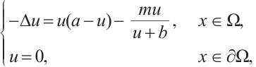
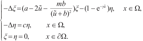
  represents the environmental carrying capacity of predators. For more detailed biological significance of the model, one can see Refs. [14-16]. Obviously, the corresponding steady-state problem to (2) can be written as
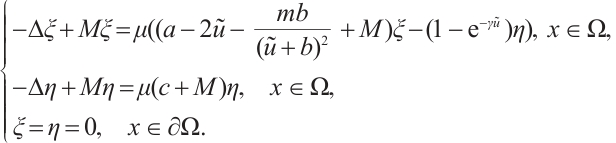
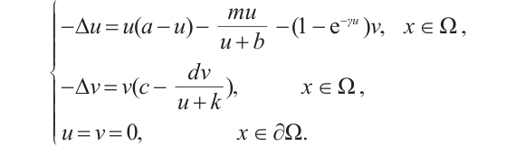 (3)
(3)
The main purpose of this paper is to clarify the influence of weak additive Allee effect and Ivlev functional response on the positive solution of model (2). The content of this paper is arranged as follows. Section 1 introduces some preliminary results. Section 2 gives the necessary conditions and prior estimates for positive solutions of (3). Section 3 gives the sufficient conditions for the existence of positive solutions of (3). Section 4 gives the uniqueness and stability of the positive solution of (3). In Section 5, the dynamics of (2) and (3) are quantitatively analyzed by numerical simulations.
1 Preliminaries
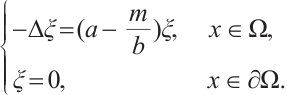
Let  . It is well known that the following problem
 (4)
(4)
has an infinite sequence of eigenvalues which are bounded below. Throughout this paper, we denote the first eigenvalue by  and the corresponding eigenfunction does not change sign on
  . We also denote that
  with the corresponding eigenfunction
  . For more detailed information, one can see Refs. [17-19].
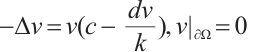
Now we consider the following boundary value problem
According to Ref. [20], if  , then u=0 is the unique non-negative solution of this problem, and it has a unique positive solution if
  . In particular, if
  and
and  , then it has a unique positive solution, denoted by
  , which is monotonically increasing with respect to
  . And then, for the boundary value problem
 (5)
(5)
using the upper and lower solution method, it has a unique positive solution  which satisfies
  when
when  and
and  . We remark here that the condition
  can meet the requirements of the condition of weak additive Allee effect, i.e.,
 . Finally, consider the following boundary value problem
 (6)
(6)
It has a unique positive solution, denoted by  , if
, if  . Moreover,
  and is monotonically decreasing with respect to
  . Especially, when
  , denote the unique positive solution by
  , that is
  .
.
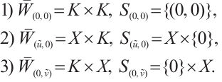
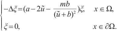
According to (5) and (6), (3) has a unique semi-trivial solution  if
if  and
and  , and has a unique semi-trivial solution
  and
and  if
if  .
.
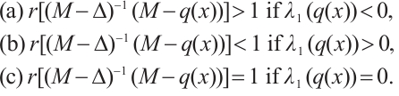
Lemma 1[21-22]
Let  ,
, with the constant
  ,
,  be the principal eigenvalue of (4). We have the following statements:
Lemma 2[22] Let  satisfy
Then there exists  such that
  for any
  .
.
2 Necessary Conditions and Prior Estimates
In this section, we use the upper and lower solution method and the strong maximum principle to establish the necessary condition and a priori estimate of positive solutions of (3).
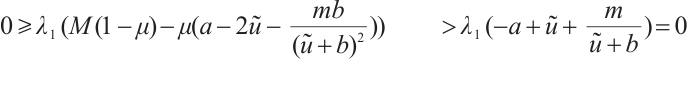
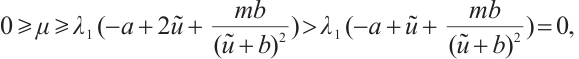
Theorem 1 If (3) has a positive solution, then  .
.
Proof Let  be a positive solution of (3). Multiply both sides of the first equation of (3) by
  and integrate on
  , we can get

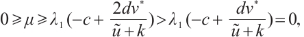
This implies that  . The inequality
  can be obtained by the second equation of (3) similarly.
Remark 1 Theorem 1 shows that when the growth rate of predator or prey is low, at least one species is extinct in (3).
Theorem 2 Suppose that  ,
, and
and  is a positive solution of (3). Then
Proof The above two inequalities are proved in the same way, and we only prove the second inequality. According to the second equation of (3) we have
If  is a positive solution of (3), according to Theorem 1 we have
  . Then
 and
and 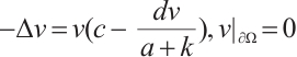
have a unique positive solution  , respectively. Thus
  can be obtained from upper-lower solution method and uniqueness of
  . The inequality
  can be obtained from the nature of
  .
.
3 Existence of Positive Steady-State Solutions
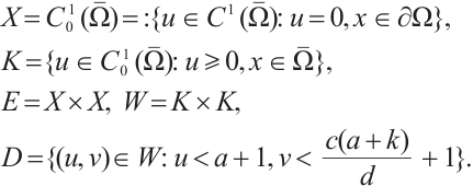
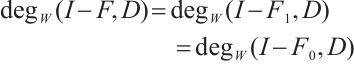
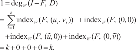
In this section, we establish the existence of positive solution of (3) by using the degree theory. In order to apply the degree theory, we make the following definitions:
Using Lemma 2, we can get
Lemma 3[22] For the mapping  . Suppose that
  is continuous on
  and
and  for any
  . If
. If  for any
  , then the topological degree
  does not depend on
  .
.
Lemma 4[22] Let  be invertible on
  .
.
(i) If  has
has  -property, then
  ;
;
(ii) If  has no
  -property, then
  , where
  is the sum of the algebraic multiplicities of the eigenvalues of
  which are larger than one.
Lemma 5 Let  . Then all eigenvalues of
  are greater than 0. Here
  is the linearization operator of (5) at
  , i.e.,
Proof By  , we have
  is a unique positive solution of (5). Thus
According to  , we have
It means that  . By the nature of principle eigenvalue, there holds
The proof is completed.
According to Theorem 2, we have any nonnegative solution of (3) belongs to  . Then there exists a positive constant
  , such that
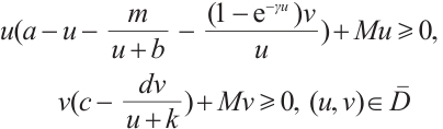
Define mapping  as
as
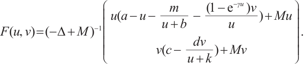 (7)
(7)
Then it is a compact operator and  . Thus
 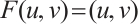 if and only if
  is a solution of (3).
For any  , we also define
Clearly,  is a positive compact operator and
  .
.
Lemma 6 Let  . We have the following statements:
(i) 
(ii) If  , then
  ,
,
(iii) If  , then
  ,
,
(iv) If  , then
  .
.
Proof (i) It is clear that  has no fixed point on
  . For any
  , the fixed point of
  is equivalent to the solution of boundary value problem
According to Theorem 2, the fixed point of  satisfies
  for any
  . Thus
  does not depend on
  from homotopic invariant property and
By the above boundary value problem has a unique solution  as
as  , we have

Notice 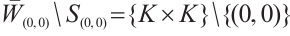 . Denote
 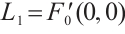 . Then
By  and Lemma 1,
  . It can derive that
  is invertible on
  and
and  has no
  -property on
  . According to Lemma 4, we have

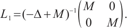
(ii) Let  . Then
At first, we will show that  is invertible on
  . If it is not true, then there is
  and
and  such that
  , i.e.,
If  , then
  , this is contrary to
  . Thus
  . Similarly,
 . This is a contradiction with
  . Then
  is invertible on
  .
.
Now we claim that  has
has  -property on
  . By
. By  and Lemma 1,
Notice that  is the principal eigenvalue of the operator
  , and the corresponding eigenfunction is
  . Take
  , then
  and
and  . Thus we have
Therefore,  has
has  -property. By Lemma 4, we have
  .
.
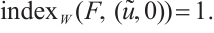
(iii) Obviously, (3) has a semi-trivial solution  . Notice that
  ,
,  , we have
  . Let
. Let  . There holds
Assume that there exists  and
and  such that
  . Then
By  , we have
  in
in  . If
. If  , then the above boundary value problem can be written as
According to  is invertible (see Lemma 5), we have
  . This contradiction leads to
  being invertible on
  .
.
By Lemma 1 and  , we also have

Notice that  is the principal eigenvalue of
  and the corresponding eigenfunction
  . Take
  , then
  . Thus
  , and
, and
It shows  has
has  -properties. According to Lemma 4, there holds
  .
.
(iv) It follows from the proof of (iii) that  is invertible on
  .
.
Now we claim  has no
  -properties on
  . If it is not true, then there exist
  and
and  such that
  . Thus
Notice that  , then
  is one eigenvalue of the
  . On the other hand, by
  and Lemma 1 we have
  , which is a contradiction.
According to  has no
  -property on
  and Lemma 4, we have
where  is the sum of the algebraic multiplicities of the eigenvalues of
  which are larger than one.
Assume that  is the eigenvalue of
  , and the corresponding eigenfunction is
  . Then
  . This can be written as
If  , then the inequality

holds from the second equation of the above boundary value problem. This is a contradiction with  . Thus
  . So
. So  . Then from the first equation of the above boundary value problem we have
This is an obvious contradiction. Therefore,  has no eigenvalue greater than one, that is
  and then
It is similar to Lemma 6 that we can get Lemma 7.
Lemma 7 Let  .
.
(i) If 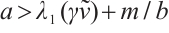 , then
 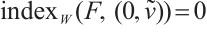 ,
,
(ii) If  , then
  ,
,
where  and
and  are given by (6) and (7), respectively.
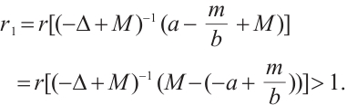
Theorem 3 If  , then (3) has at least one positive solution.
Proof From the additivity of the degree, combining Lemma 6 and Lemma 7 we have
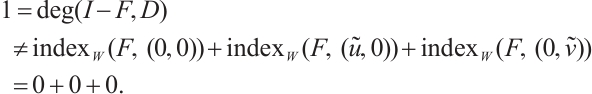
Therefore, (3) has at least one positive solution.
Remark 2 Theorem 3 shows that predator and prey can coexist as long as the Allee effect constant satisfies the appropriate conditions and the growth rates of predator and prey are appropriately large.
4 Uniqueness and Stability
In this section, we use the stability theory of linear operators to discuss uniqueness and stability of positive steady-state solutions. First, the following Lemma 8 is given.
Lemma 8 Let  . There exists a constant
  small enough, such that any positive solution of (3) is nondegenerate and linearly stable when
  (if the positive solution exists).
Proof Assume that it is not true. For  with
with  , there exists a sequence of positive solutions
  of (3), which are degenerate or unstable.
Now we suppose there are  and
and  , which satisfy
  and
and  , such that
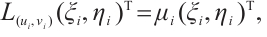
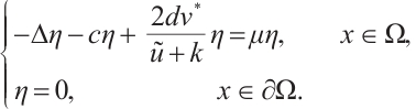
where  is the linearization operator of (3) at
  , i.e.,
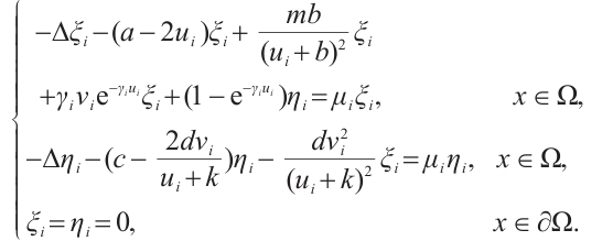 (8)
(8)
Obviously, 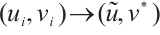 as
as  , where
  is a unique positive solution of the boundary value problem
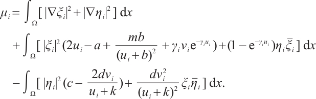
Multiplying  and
and  both sides of the first and second equations in (8), respectively, then integrating on
  and adding the results, we can get
Note that  ,
,  and
and  are both bounded according to Theorem 2. Thus
  is also bounded. Suppose
  (take subsequences if necessary). By
  estimates for (8), both
  and
and  are also bounded in
  for
for  . So there exists a convergent subsequence of
  , which is still denoted by
  for the sake of convenience, such that
  in
in  . Taking the limit in (8) with respect to
  , then
  satisfies
 (9)
(9)
under the condition of weak convergence. According to the regularity theory,  is a pair of classical solution of (9). It means that
  is a real number and
  .
.
If  , then
  is an eigenvalue of the problem
Combining with Lemma 5, there holds
which is a contradiction. Thus  and (9) can be written as
Similarly, if  , then
also a contradiction. So  , which is a new contradiction with
 .
.
Theorem 4 Let 
 and
and  be a positive constant small enough, then (3) has a unique non-degenerate and linearly stable positive solution if
  .
.
Proof By Theorem 3 and Lemma 8, the existence of positive solution is clear. So we only show the rest of this Theorem.
At first, it is easy to verify that both trivial solution  and semi-trivial solutions
  are all non-degenerate, linearly stable and isolated. According to the compactness theory[23], (3) has at most a finite number of positive solutions, which are recorded as
  . It is similar to the proof of Lemma 8 that
  is invertible on
  . Notice that
  , we have
  . Thus
  has no
  -property.
Furthermore,  has no eigenvalue which is greater than 1. According to Lemma 4,
 . From the additivity of degree and combining Lemma 6 and Lemma 7, we have
It follows that  . The uniqueness of the positive solution is obtained.
Remark 3 Theorem 4 shows that, as long as the Allee effect constant satisfies the appropriate relationship and the growth rate of predator and prey is appropriately large, the predator and prey not only coexist, but also the coexistence mode generated by low predator efficiency is stable.
5 Numerical Simulations
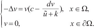
In this section, some numerical simulations for (2) and (3) in one-dimensional  will be carried out to verify the qualitative results of this paper. The algorithm used here is Pdepe in MATLAB. The initial value is taken as
 (10)
(10)
where  is a positive constant. The principal eigenvalue of
  under the homogeneous Dirichlet boundary conditions is
  when
when  [24]. By the property of the principal eigenvalue we have
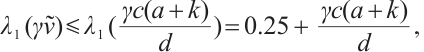
and
 only if
(i) Existence of steady-state solutions
As is well known, when the solution of (2) does not change with time, it is called the steady-state solution of (2), which is the solution of (3). The other remark here is that the weak Allee effect constant relationship  can be satisfied when
  . A large number of numerical simulations are consistent with Theorem 3. Some examples are provided in the following statements, where the parameters are given by

Let  . (3) has a unique solution
  , which is shown in Fig. 1.
 |
Fig. 1 Steady-state solution 
|
Let  . (3) has a unique semi-trivial solution
  , which is shown in Fig. 2.
 |
Fig. 2 Steady-state solution 
|
Let  . (3) has a unique semi-trivial solution
  , which is shown in Fig. 3.
 |
Fig. 3 Steady-state solution 
|
Let  , (3) has a positive solution
  , which is shown in Fig. 4.
 |
Fig. 4 Steady-state solution 
|
(ii) Influence of  on the positive steady-state solutions
A large number of numerical simulations will verify the existence of steady-state solution when  is sufficiently small. One of examples is shown in Fig. 5, which is consistent with the existence of positive solution in Theorem 4, where the parameters take
 (11)
(11)
 |
Fig. 5 Existence of steady-state solutions, 
|
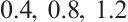
Furthermore, a large number of numerical simulations show that predator and prey density decrease with the increase of predation rate  . One of the examples is shown in Fig. 6, where
  and the other parameters are given by (11).
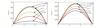 |
Fig. 6 Existence of steady-state solutions,  and and 
|
In addition, our numerical simulations show that under appropriate parameters, (3) has still the positive steady-state solution even if the  is large, which needs to be theoretically proved in future research. One example is shown in Fig. 7, where the parameters take

 (12)
(12)
 |
Fig. 7 Existence of steady-state solutions, 
|
(iii) Influence of  on the stability of positive steady-state solutions
We change the initial value parameter  to simulate the disturbance of the initial value. For the convenience of discussion, the maximum norm of
  with respect to
  (denote it by
  ) is plotted by Pdepe. If
  and
and  do not change with initial values after a long period of time, then
  and
and  are stable. Otherwise, the steady-state solution is unstable. In fact, a large number of numerical simulations show that a positive steady-state solution is stable regardless of whether the
  is large or small.
For example, let  and
and 
 , the other parameters are given by (11), see Fig. 8. This shows that the positive solution is stable, which is consisted with the stability of positive solution in Theorem 4.
 |
Fig. 8 Stability of steady-state solutions, 
|
Let  and
and 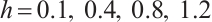 , the other parameters are given by (12), see Fig. 9. This shows that the positive solution is also stable, but the theoretical proof of this conclusion needs to be studied further.
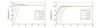 |
Fig. 9 Stability of steady-state solutions, 
|
6 Conclusion
We simulate the interaction between invertebrates and plankton using a modified Leslie-Gower predator-prey model with the Ivlev type functional response function, which is used to describe the fact that Tortanus dextrilubatus prey on zooplankton. Meanwhile, we also focus on the Allee effect in the model. Our research shows that under the Allee effect, predators and prey can coexist. Specifically, the growth rates of predators and prey can control the uniqueness of the coexistence pattern, which is consistent with the actual situation. We employ some numerical simulations primarily to verify the rationality of the conditions in this article, such as Lemma 8 and Theorem 4, etc. At the same time, we also verify the stability of the steady-state solutions by making small perturbations to the initial values. In a sense, these studies only provide a framework for model dynamics, and there are still some things that have not been studied, such as simulating the non-enclosure of habitats using Neumann boundary conditions, then the properties of constant and non-constant solutions of the model will be an interesting problem. In fact, more complex coexistence patterns of predator-prey systems can be examined through Turing pattern and Hopf bifurcation.
References
- Zhang C H, Yang W B. Dynamic behaviors of a predator-prey model with weak additive Allee effect on prey[J]. Nonlinear Analysis: Real World Applications, 2020, 55: 103137. [Google Scholar]
- Aguirre P, González-Olivares E, Sáez E. Three limit cycles in a Leslie-Gower predator-prey model with additive Allee effect[J]. SIAM Journal on Applied Mathematics, 2009, 69(5): 1244-1262. [Google Scholar]
- Cai Y L, Banerjee M, Kang Y, et al. Spatiotemporal complexity in a predator: Prey model with weak Allee effects[J]. Mathematical Biosciences and Engineering, 2014, 11(6): 1247-1274. [Google Scholar]
- Pal P J, Mandal P K. Bifurcation analysis of a modified Leslie-Gower predator-prey model with Beddington-DeAngelis functional response and strong Allee effect[J]. Mathematics and Computers in Simulation, 2014, 97: 123-146. [Google Scholar]
- Yang W S, Li Y Q. Dynamics of a diffusive predator-prey model with modified Leslie-Gower and Holling-type Ⅲ schemes[J]. Computers & Mathematics with Applications, 2013, 65(11): 1727-1737. [Google Scholar]
- Yang W B. Analysis on existence of bifurcation solutions for a predator-prey model with herd behavior[J]. Applied Mathematical Modelling, 2018, 53: 433-446. [Google Scholar]
- Li S B, Wu J H, Dong Y Y. Uniqueness and stability of a predator-prey model with C-M functional response[J]. Computers & Mathematics with Applications, 2015, 69(10): 1080-1095. [Google Scholar]
- Hooff R C, Bollens S M. Functional response and potential predatory impact of Tortanus dextrilobatus, a carnivorous copepod recently introduced to the San Francisco Estuary[J]. Marine Ecology Progress Series, 2004, 277: 167-179. [Google Scholar]
- Wang X C, Wei J J. Dynamics in a diffusive predator-prey system with strong Allee effect and Ivlev-type functional response[J]. Journal of Mathematical Analysis and Applications, 2015, 422(2): 1447-1462. [Google Scholar]
- Wang H L, Wang W M. The dynamical complexity of a Ivlev-type prey-predator system with impulsive effect[J]. Chaos, Solitons & Fractals, 2008, 38(4): 1168-1176. [Google Scholar]
- Wang X C, Wei J J. Diffusion-driven stability and bifurcation in a predator-prey system with Ivlev-type functional response[J]. Applicable Analysis, 2013, 92(4): 752-775. [Google Scholar]
- Li S B, Wu J H, Nie H. Steady-state bifurcation and Hopf bifurcation for a diffusive Leslie-Gower predator-prey model[J]. Computers & Mathematics with Applications, 2015, 70(12): 3043-3056. [Google Scholar]
- Zhou J, Shi J P. The existence, bifurcation and stability of positive stationary solutions of a diffusive Leslie-Gower predator–prey model with Holling-type Ⅱ functional responses[J]. Journal of Mathematical Analysis and Applications, 2013, 405(2): 618-630. [Google Scholar]
- Cai Y L, Zhao C D, Wang W M, et al. Dynamics of a Leslie-Gower predator-prey model with additive Allee effect[J]. Applied Mathematical Modelling, 2015, 39(7): 2092-2106. [Google Scholar]
- Yang L, Zhong S M. Dynamics of a diffusive predator-prey model with modified Leslie-Gower schemes and additive Allee effect[J]. Computational and Applied Mathematics, 2015, 34(2): 671-690. [Google Scholar]
- Ma Z P. Spatiotemporal dynamics of a diffusive Leslie-Gower prey-predator model with strong Allee effect[J]. Nonlinear Analysis: Real World Applications, 2019, 50: 651-674. [Google Scholar]
- Wang L J, Jiang H L. Properties and numerical simulations of positive solutions for a variable-territory model[J]. Applied Mathematics and Computation, 2014, 236: 647-662. [Google Scholar]
- Cano-Casanova S. Existence and structure of the set of positive solutions of a general class of sublinear elliptic non-classical mixed boundary value problems[J]. Nonlinear Analysis: Theory, Methods & Applications, 2002, 49(3): 361-430. [Google Scholar]
- Blat J, Brown K J. Global bifurcation of positive solutions in some systems of elliptic equations[J]. SIAM Journal on Mathematical Analysis, 1986, 17(6): 1339-1353. [Google Scholar]
- Ye Q X, Li Z Y, Wang M X, et al. Introduction to Reaction-Diffusion Equation[M]. Beijing: Science Press, 2013(Ch). [Google Scholar]
- Pao C V. Nonlinear Parabolic and Elliptic Equations[M]. Cham: Springer-Verlag, 1992. [Google Scholar]
- Wang M X. Nonlinear Elliptic Equation[M]. Beijing: Science Press, 2007(Ch). [Google Scholar]
- Du Y H, Lou Y. Some uniqueness and exact multiplicity results for a predator-prey model[J]. Transactions of the American Mathematical Society, 1997, 349(6): 2443-2475. [Google Scholar]
- Wang L J, Jiang H L. The multiplicity and uniqueness of positive solutions for a competition model with diffusion[J]. Journal of Wuhan University (Natural Science Edition), 2015, 61(4): 308-314(Ch). [Google Scholar]
All Figures
|
Fig. 1 Steady-state solution
|
| In the text | |
|
Fig. 2 Steady-state solution
|
| In the text | |
|
Fig. 3 Steady-state solution
|
| In the text | |
|
Fig. 4 Steady-state solution
|
| In the text | |
|
Fig. 5 Existence of steady-state solutions,
|
| In the text | |
|
Fig. 6 Existence of steady-state solutions, and
|
| In the text | |
|
Fig. 7 Existence of steady-state solutions,
|
| In the text | |
|
Fig. 8 Stability of steady-state solutions,
|
| In the text | |
|
Fig. 9 Stability of steady-state solutions,
|
| In the text | |
Current usage metrics show cumulative count of Article Views (full-text article views including HTML views, PDF and ePub downloads, according to the available data) and Abstracts Views on Vision4Press platform.
Data correspond to usage on the plateform after 2015. The current usage metrics is available 48-96 hours after online publication and is updated daily on week days.
Initial download of the metrics may take a while.