


| Issue |
Wuhan Univ. J. Nat. Sci.
Volume 31, Number 3, June 2026
|
|
|---|---|---|
| Page(s) | 250 - 254 | |
| DOI | https://doi.org/10.1051/wujns/2026313250 | |
| Published online | 24 June 2026 | |
Mathematics
CLC number: O175.2
Global Strong Solutions to a Two-Dimensional Keller-Segel-Navier-Stokes System with Subcritical Sensitivity
具有次临界敏感性的二维Keller-Segel-Navier-Stokes方程组的强解的整体存在性
1
Department of Mathematics and Physics, Sanjiang University, Nanjing 210012, Jiangsu, China
(三江学院 数理部,江苏 南京 210012)
2
School of Mathematics, Nanjing University of Aeronautics and Astronautics, Nanjing 211106, Jiangsu, China
(南京航空航天大学 数学学院,江苏 南京 211106)
3
School of Mathematics and Big Data, Chaohu University, Hefei 238000, Anhui, China
(巢湖学院 数学与大数据学院,安徽 合肥 238000)
4
School of Mathematics, Southeast University, Nanjing 211189, Jiangsu, China
(东南大学 数学学院,江苏 南京 211189)
† Corresponding author. E-mail: This email address is being protected from spambots. You need JavaScript enabled to view it.
Received:
8
November
2025
Abstract
In this paper, we prove the global existence of strong solutions to a two-dimensional (2D) Keller-Segel-Navier-Stokes system with subcritical sensitivity in a bounded domain. Using energy methods, interpolation inequalities and the Gronwall lemma, we establish uniform a priori estimates for the solutions. We prove the existence and uniqueness of global strong solutions under appropriate initial conditions, along with higher-order Sobolev regularity of solutions. The result extends existing conclusions and enriches the global well-posedness theory for chemotaxis-fluid coupled models.
摘要
本文证明了有界区域中一类带次临界敏感性的二维 Keller-Segel-Navier-Stokes 系统强解的整体存在性。利用能量方法、插值不等式及 Gronwall 引理,我们建立了解的一致先验估计。在适当的初值条件下,证明了该系统整体强解的存在唯一性,并得到了解的高阶 Sobolev 正则性。该结果推广了已有的结论,丰富了趋化–流体耦合模型的整体适定性理论。
Key words: chemotaxis / Keller-Segel-Navier-Stokes / strong solutions
关键字 : 趋化性 / Keller-Segel-Navier-Stokes方程 / 强解
Cite this article: LU Shengqi, CHEN Miaochao, LIU Qilin. Global Strong Solutions to a Two-Dimensional Keller-Segel-Navier-Stokes System with Subcritical Sensitivity[J]. Wuhan Univ J of Nat Sci, 2026, 31(3): 250-254.
Biography: LU Shengqi, male, Ph. D. candidate, Associate professor, research direction: partial differential equations. E-mail: This email address is being protected from spambots. You need JavaScript enabled to view it.
Foundation item: Supported by the National Natural Science Foundation of China (12171459) and the Key Project of University Natural Science of Anhui Province ( 2023AH052096)
© Wuhan University 2026
 This is an Open Access article distributed under the terms of the Creative Commons Attribution License (https://creativecommons.org/licenses/by/4.0), which permits unrestricted use, distribution, and reproduction in any medium, provided the original work is properly cited.
0 Introduction
We consider the following model of a Keller-Segel-Navier-Stokes with subcritical sensitivity[1-2]:
 (1)
(1)
 (2)
(2)
 (3)
(3)
 (4)
(4)
 (5)
(5)
 (6)
(6)
 (7)
(7)
where  is the velocity of the fluid,
  is the pressure,
  and
and  denote the density of amoebae, oxygen and chemical attractant, respectively. The smooth function
  is a potential.
  is the chemotactic sensitivity.
  is a bounded convex domain with smooth boundary
  ,
,  is the unit outward normal vector to
  .
.
The two-dimensional Keller-Segel-Navier-Stokes system serves as a fundamental mathematical model for characterizing the dynamic evolution of chemotactic biological populations in fluid environments[3-4]. Its physical foundation stems from bidirectional coupling between chemotactic behavior and fluid motion: biological entities form aggregation patterns through sensing chemical concentration gradients (Keller-Segel mechanism), while viscous fluid flow (Navier-Stokes equations) alters population distribution via turbulent or laminar transport. The subcritical sensitivity condition further regulates biological response intensity to prevent solution blowup. This study establishes the theoretical conditions ensuring global existence of strong solutions for the two-dimensional Keller-Segel-Navier-Stokes system under the subcritical sensitivity condition in bounded domains. Beyond providing a supplementary analytical approach for chemotaxis-fluid systems, the research advances understanding of nonlinear stability mechanisms in biological-fluid interactions through energy estimation methods for coupled systems. Its practical significance lies in offering theoretical support for biomedical and environmental engineering applications, including tumor cell migration modeling, algal bloom prediction, and microfluidic chip design. Methodologically, the developed techniques for a priori estimates and compactness arguments provide transferable mathematical tools for interdisciplinary research in magnetohydrodynamics and other complex systems.
Recent advances in mathematical modeling of chemotaxis-fluid systems have yielded significant insights. Bellomo et al[5] conducted a comprehensive analysis of Keller-Segel models and their modifications, deriving macroscopic formulations through kinetic theory that prevent non-physical solution blow-up. Kiselev and Ryzhik[6] demonstrated that chemotactic interactions can achieve near-complete biological reaction efficiency (>99%), with this enhancement being independent of reaction amplitude, thereby revealing fundamental nonlinear coupling mechanisms. In two-dimensional domains, Wang et al[7] established global weak solution existence for the chemotaxis-Navier-Stokes system under subcritical sensitivity conditions ( ), providing methodological foundations for our strong solution analysis. For three-dimensional cases, Fan and Li[8] proved vanishing viscosity limits using
  -energy methods, though their approach did not address stability regulation by subcritical parameters. This study presents a proof of global strong solution existence for two-dimensional systems with subcritical sensitivity (where
  denotes the chemotactic sensitivity coefficient and
  is the critical threshold, satisfying
  ) in bounded domains. Through hierarchical energy estimates and Poincaré inequality control, we reveal the deterministic role of subcritical conditions in maintaining system stability.
When  , system (3), (4) and (5) reduces to the Keller-Segel system[9-11], which received many studies[12-18].
Fan and Zhao[19] established some regularity criteria when  .
.
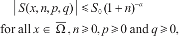
We assume that 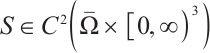 has the property that there exist
  and
and  fulfilling
 (8)
(8)
where we evidently may assume without loss of generality that  .
.
When  , Wang et al[7] showed the global existence of strong solutions.
The aim of this paper is to generalize the results in Ref. [7] to the case  , we will prove
Theorem 1 Let 
 in
in  and
and 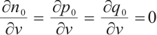 on
on  . Suppose that
  is a smooth function and (8) holds true. Then the problem (1)-(7) has a unique strong solution
  satisfying
 (9)
(9)
for any given  .
.
1 Proof of Theorem 1
This section is devoted to the proof of Theorem 1. It is easy to show the local well-posedness of smooth solutions, we only need to prove some a priori estimates (9).
First, by the maximum principle, and integrating (3) over  we get
 (10)
(10)
Integrating (5) over Ω, we see that

which gives
 (11)
(11)
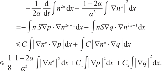
Testing (3) by  , using (2) and (8), we find that
 (12)
(12)
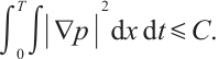
Testing (4) by  and using (2) and (10), we deduce that

which yields
 (13)
(13)
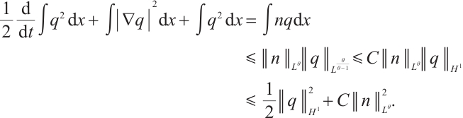
Testing (5) by  and using (2), we infer that
 (14)
(14)
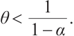
On the other hand, we first impose the condition that
 (15)
(15)
Then, by applying Young's inequality under this constraint, we observe that

 (16)
(16)
Summing up (12) and (14), using (13), (16) and the Gronwall inequality, we have
 (17)
(17)
Using the Gagliardo-Nirenberg inequality and (17), we have
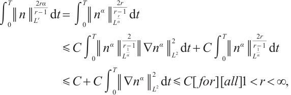 (18)
(18)
and
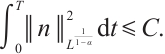 (19)
(19)
Testing (1) by  and using (2) and (19), we have
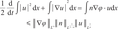

which implies
 (20)
(20)
Testing (5) by 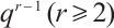 and using (2), (18) and by the same calculations as those in Ref. [5], we have
 (21)
(21)
We omit the details here.
Testing (3) by  , using (2), and by the same calculations as that in Ref. [5], we have
 (22)
(22)
 (23)
(23)
and hence we omit the details here.
Using (23), testing (1) by  we easily get
 (24)
(24)
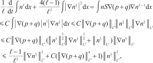
Testing (3) by 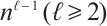 , using (2) and (22), we have
which gives
 (25)
(25)
By the standard  -estimate of heat equations, it follows from (5), (25) and (24) that
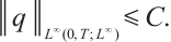 (26)
(26)
It follows from (4), (5), (22) and (24) that
 (27)
(27)
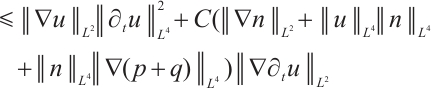
Applying  to (1), testing by
  , using (2), (3), (24), (25) and (22), we have





which leads to
 (28)
(28)
And thus
 (29)
(29)
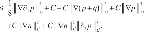
Applying  to (4), testing by
  , using (2), (10), (28), (29), (25) and (22), we have






which gives
 (30)
(30)
and hence
 (31)
(31)
Similarly to (30)-(31), we have
 (32)
(32)
 (33)
(33)
Similarly to (26), we have
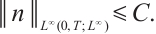 (34)
(34)
Now testing (3) by  it is easy to verify that
 (35)
(35)
we omit the details here.
Applying  to (3), testing by
  , using (2), (34), (35) and (28)-(33), we arrive at







which implies
 (36)
(36)
whence
 (37)
(37)
This completes the proof.
References
- Kozono H, Miura M, Sugiyama Y. Existence and uniqueness theorem on mild solutions to the Keller-Segel system coupled with the Navier-Stokes fluid[J]. Journal of Functional Analysis, 2016, 270(5): 1663-1683. [Google Scholar]
- Kozono H, Miura M, Sugiyama Y. Time global existence and finite time blow-up criterion for solutions to the Keller-Segel system coupled with the Navier-Stokes fluid[J]. Journal of Differential Equations, 2019, 267(9): 5410-5492. [Google Scholar]
- Winkler M. Small-Mass solutions in the two-dimensional Keller-Segel system coupled to the Navier-Stokes equations[J]. SIAM Journal on Mathematical Analysis, 2020, 52(2): 2041-2080. [Google Scholar]
- Chen M C, Chen F Q, Lu S Q. A logarithmic extensibility criterion for a Keller-Segel-Navier-Stokes system in a bounded domain[J]. Journal of Mathematical Physics, Analysis, Geometry, 2025, 21(2): 179-202. [Google Scholar]
- Bellomo N, Bellouquid A, Tao Y, et al. Toward a mathematical theory of Keller-Segel models of pattern formation in biological tissues[J]. Mathematical Models and Methods in Applied Sciences, 2015, 25(9): 1663-1763. [Google Scholar]
- Kiselev A, Ryzhik L. Biomixing by chemotaxis and enhancement of biological reactions[J]. Communications in Partial Differential Equations, 2012, 37(2): 298-318. [Google Scholar]
- Wang Y L, Winkler M, Xiang Z Y. Global classical solutions in a two-dimensional chemotaxis-Navier-Stokes system with subcritical sensitivity[J]. Annali Scuola Normale Superiore - Classe Di Scienze, 2018, 18(5): 421-466. [Google Scholar]
- Fan J S, Li F C. Vanishing viscosity limits of a chemotaxis-Navier-Stokes model[J]. Acta Mathematicae Applicatae Sinica, English Series, 2025, 41(4): 1156-1166. [Google Scholar]
- Keller E F, Segel L A. Initiation of slime mold aggregation viewed as an instability[J]. Journal of Theoretical Biology, 1970, 26(3): 399-415. [Google Scholar]
- Keller E F, Segel L A. Model for chemotaxis[J]. Journal of Theoretical Biology, 1971, 30(2): 225-234. [Google Scholar]
- Keller E F, Segel L A. Traveling bands of chemotactic bacteria: A theoretical analysis[J]. Journal of Theoretical Biology, 1971, 30(2): 235-248. [Google Scholar]
- Biler P. Global solutions to some parabolic-elliptic systems of chemotaxis[J]. Advances in Applied Mathematics, 1999, 9(1): 347-359. [Google Scholar]
- Corrias L, Perthame B, Zaag H. Global solutions of some chemotaxis and angiogenesis systems in high space dimensions[J]. Milan Journal of Mathematics, 2004, 72(1): 1-28. [Google Scholar]
- Hillen T, Painter K J. A user's guide to PDE models for chemotaxis[J]. Journal of Mathematical Biology, 2009, 58(1): 183-217. [Google Scholar]
- Horstmann D. From 1970 until present: The Keller-Segel model in chemotaxis and its consequences: I[J]. Jahresbericht der Deutschen Mathematiker-Vereinigung, 2003, 105(3):103-165. [Google Scholar]
- Sleeman B D, Ward M J, Wei J C. The existence and stability of spike patterns in a chemotaxis model[J]. SIAM Journal on Applied Mathematics, 2005, 65(3): 790-817. [Google Scholar]
- Winkler M. Global solutions in a fully parabolic chemotaxis system with singular sensitivity[J]. Mathematical Methods in the Applied Sciences, 2011, 34(2): 176-190. [Google Scholar]
- Wrzosek D. Long-time behaviour of solutions to a chemotaxis model with volume-filling effect[J]. Proceedings of the Royal Society of Edinburgh: Section A Mathematics, 2006, 136(2): 431-444. [Google Scholar]
- Fan J S, Zhao K. Improved extensibility criteria and global well-posedness of a coupled chemotaxis-fluid model on bounded domains[J]. Discrete and Continuous Dynamical Systems - B, 2018, 23(9): 3949-3967. [Google Scholar]
Current usage metrics show cumulative count of Article Views (full-text article views including HTML views, PDF and ePub downloads, according to the available data) and Abstracts Views on Vision4Press platform.
Data correspond to usage on the plateform after 2015. The current usage metrics is available 48-96 hours after online publication and is updated daily on week days.
Initial download of the metrics may take a while.