| Issue |
Wuhan Univ. J. Nat. Sci.
Volume 27, Number 4, August 2022
|
|
|---|---|---|
| Page(s) | 321 - 330 | |
| DOI | https://doi.org/10.1051/wujns/2022274321 | |
| Published online | 26 September 2022 | |
Mathematics
CLC number: F 48
Optimal Investment Strategy of Defined Contribution Pension Based on Bequest Motivation and Loss Aversion
School of Mathematics and Finance, Anhui Polytechnic University, Wuhu 241000, Anhui, China
Received:
11
May
2022
Abstract
Under the S-shaped utility of loss aversion, this paper considers the bequest motivation of pension plan participants, random salary income before retirement and the substitution rate between receiving pension benefits after retirement and wages before retirement, and studies the optimal investment strategy of defined contribution (DC) pension. Assuming that pension funds can invest in a financial market consisting of three assets (risk-free asset cash, rolling bonds and stocks), inflation is considered by discount. Under the S-shaped utility, the Lagrange method is used to find the terminal optimal surplus of pensions in retirement, so as to find the terminal optimal wealth, and then the martingale method is used to find the optimal wealth process and investment strategy. Finally, a sensitivity analysis is carried out on the the influence of bequest motivation and loss aversion on the optimal investment strategy of DC pension.
Key words: bequest motivation / loss aversion / substitution rate / inflation / martingale method / investment strategy
Biography: XUE Juan, female, Master candidate, research direction: risk management. E-mail: This email address is being protected from spambots. You need JavaScript enabled to view it.
Fundation item: Supported by the National Social Science Foundation of China (20BTJ048), and Anhui University Humanities and Social Science Research Major Project (SK2021ZD0043)
© Wuhan University 2022
 This is an Open Access article distributed under the terms of the Creative Commons Attribution License (https://creativecommons.org/licenses/by/4.0), which permits unrestricted use, distribution, and reproduction in any medium, provided the original work is properly cited.
0 Introduction
Pension insurance plan is a crucial part of the current social security system, which is related to the basic living standard and quality of the people after retirement. China is the country with the largest population in the world, with a huge scale of pensions. As of 2020, there are 998.65 million people participating in pension insurance across the country, an increase of 31.11 million people compared to 2019. In 2020, the annual income of pension funds was 492 million yuan, with a cumulative balance of 5.81 trillion yuan. In the face of such a huge pension fund, how to optimize the asset allocation of pension fund is particularly important for pension managers.
There are two main types of endowment insurance: defined benefit (DB) and defined contribution (DC). DB pension plan participants receive a fixed pension after retirement, and fund managers bear investment risks. Different from DB pensions, DC pension participants regularly deposit a certain amount by establishing personal accounts. Fund managers accumulate benefits for pension participants by investing in the financial market, and the risks are borne by the participants themselves. Therefore, the asset allocation of DC pensions is particularly important. In recent years, there has been extensive research on DC pension asset allocation in the actuarial field. Boulier et al[1] studied the DC pension asset allocation model under constant interest rate risk, and under the constant relative risk averse (CRRA) utility function, the terminal wealth in the model should ensure that the pension participants' normal living standards after retirement are met. Gao[2] used the constant elasticity of variance (CEV) model to describe the stock price, applied stochastic optimal control, power transformation and variable replacement techniques, and deduced the explicit solutions of the CRRA utility function and the constant absolute risk aversion (CARA) utility function, respectively. Zhang et al[3] used an affine model to find the equilibrium investment strategy of the DC pension plan under the mean-variance criterion in which both interest rates and volatility are random in the financial market.
DC pension plan generally has a long term. With the continuous development of financial market, pension managers have to consider the risk of inflation. In recent years, more and more scholars have focused on inflation risk to pension managerment. Tiro et al[4] studied the optimal investment strategy of DC pension by applying dynamic programming to Hamilton-Jacobi-Bellman (HJB) equation under stochastic interest rate and inflation risk. Wang et al[5] assumed that risky assets obeyed the O-U process, also considered stochastic income and inflation risks, and used the stochastic control method to derive the HJB equation to study the optimal asset allocation of DC pensions. Han et al[6] used stochastic dynamic programming method to study the use of index bonds to hedge inflation risk under the utility of CRRA, and obtained the explicit solution of the optimal investment strategy. Wu et al[7] considered the inflation risk and wage risk, and studied the optimal investment strategy of the DC pension plan under the mean-variance criterion, gave the HJB equation, and used the stochastic control technology to obtain the closed-form time-consistent investment strategy and explicit solution to the equilibrium efficient frontier. Baltas et al[8] studied the optimal management of defined contribution pension funds in the allocation stage under the influence of inflation, mortality and model uncertainty, and clarified the impact of robustness and inflation on optimal investment decisions.
In addition, as the fertility rate decreases with the aging population, Hou et al[9] considered the existence range and determinants of bequest motivation based on the data of the China Household Finance Survey, and studied the influence of bequest motivation on household consumption and asset allocation decisions. The results of the analysis show that more than 90% of urban families in China have bequest motivations, and the families with older age, higher income, more children and sons are more likely to have bequest motivations. Choi et al[10] investigated the relationship between financial assets and bequest expectations. Their samples included 10 340 middle-aged and older Americans from the 2014 Health and Retirement Study. The results of the ordinary least squares regression model showed that there was a positive correlation between bequest expectations and a negative correlation between depression and bequest expectations. Shi et al[11] considered the bequest motivation of pension plan participants, the random wage flow before retirement and the minimum living guarantee after retirement under the CRRA utility function, and used the Lagrange method to solve the optimal surplus at the terminal time of DC pension, and then adopted the martingale method to get the optimal wealth process and investment strategy.
The above literatures all consider the optimal investment strategy of DC pension under the CRRA utility function, and believe that fund managers always have a relatively constant attitude towards risk. However, different fund managers are always different towards risk and the same losses and gains. A CRRA-type preference would result in a significant portion of wealth being invested in equities, which is too risky for pension funds. Furthermore, according to the prospect theory proposed by Kahneman and Tversk[12], most investors are loss averse and have two behavioral characteristics. First, the investor does not focus on the absolute level of wealth itself, but on the gain and loss relative to a predetermined reference point, which can be interpreted as the goal of his standard of living. Second, losses generally cause more discomfort to investors, who are more sensitive to losses than gains. Guan and Liang[13] assumed that the interest rate obeyed the O-U model and considered stock price volatility, requiring fund managers to study the optimal asset allocation of DC pensions under the constraints of loss aversion and value at risk (VaR). Chen et al[14] studied the optimal investment strategy of DC pensions under loss aversion utility, taking into account the inflation risk, longevity risk and random income risk that pension participants may face. Wang et al[15] considered that the pension participants were loss-averse on the basis of considering the inflation risk, and used the S-shaped utility function and martingale method to deduce the explicit solution of the optimal investment of the pension participants at any time before retirement.
Through the above literature analysis, it is found that inflation, bequest motivation and loss aversion are all important factors affecting the optimal asset allocation of DC pensions.
With the development of economy and the improvement of living standards, in addition to the demand of basic life safeguard, pension participants after retirement have more requirement for the pursuit of spiritual life, such as traveling after retiring, raising a lovely pets and so on, which needs higher retirement welfare support. Therefore, we take into account the replacement rate between the pension benefits that participants can receive after retirement and their wages before retirement into the model, which is more in line with the actual life of current workers after retirement and also has certain practical significance at the same time. This paper adopts the S-shaped utility function on the basis of the above model, considers the stochastic interest rate risk, inflation risk, longevity risk and bequest motivation to study the optimal investment strategy of DC pension, and introduces the substitution rate between receiving pension benefits after retirement and wages before retirement and bequest motivation on the basis of Wang et al[15].
1 Methodology
1.1 Financial Market
The financial market studied in this paper is a continuous, frictionless and arbitrage-free complete market. Suppose the market consists of three assets, a risk-free asset, an index bond, and a risky asset, and the pension plan starts at time 0,  indicating the time of retirement.
Define a complete probability space  , where
  is the real world,
  represents all the information available in the market up to time t , P is the real world probability.
  is the standard Brownian motion of dimension, and
  and
and  are independent of each other.
The risk-free asset price  at time
  satisfies the following differential equation:
 (1)
(1)
where  is a random interest rate satisfying the O-U model:
 (2)
(2)
where  and are all constants.
The price  of a zero-interest bond with maturity
  satisfies the following differential equation at time
  :
:
 (3)
(3)
where  ,
,  represents the risky market price of
  ,
,  represents the volatility of
  . Boulier et al[1] mentioned that all zero-interest bonds cannot be found in a real market, where rolling bonds and cash can replicate arbitrary zero-interest bonds, so interest rate risk is hedged by a rolling bond with a constant maturity date
  .
.
The price  to buy a rolling bond with a fixed maturity constant
  satisfies the following stochastic differential equation:
 (4)
(4)
Rolling bonds and cash can get a zero-interest bond using the following relational combination:
 (5)
(5)
The price  of a risky asset stock at time
  obeys the following stochastic differential equation:
 (6)
(6)
where  and both are constants,
  is the risk-reward price of
  .
.
Since the pension plan has a longer investment period, the impact of inflation is more significant. Considering the inflation rate, the following stochastic differential equation is satisfied:
 (7)
(7)
where  is the expected inflation index;
  is inflation matrix. They are all measurable, uniformly bounded processes on
To eliminate the impact of inflation, we divided the nominal price of stocks by the inflation rate to get the real stock price as:
 (8)
(8)
Applying Ito's Lemma, it is obtained that  satisfies the following stochastic differential equation:
 (9)
(9)
where

Pension participants will continuously contribute a certain amount of insurance money to their personal pension accounts, and the amount of money contributed to the pension fund at time t equals the salary multiplies a certain contribution rate. It is assumed that the salary income of pension  of participants during the pension plan satisfies the following geometric Brownian motion:
 (10)
(10)
where  and
and  are all constants greater than zero,
1.2 Wealth Process and Surplus Process
Assume that the initial amount of the pension account is  and the contribution rate of the pension participant is constant
  .
.  and
and  are the proportion of investment in rolling bonds and stocks of risky assets and cash of risk-free assets, respectively, set
  , then the wealth process of pension account
  satisfies:
 (11)
(11)
where  represents the initial value of wealth, and c represents the salary contribution rate of pension scheme participants.

In actual life, pension plan participants gave money to pension managers for capital investment and accumulation, but the risk is borne by themselves. The investment risk of failure may lead to the low level of retirement pension accounts wealth, therefore pension participants are more concerned about the substitution rate between receiving pension benefits after retirement and wages before retirement, so we consider setting up the model for post-retirement pension benefits
where  is the ratio of the level monthly payout of the pension fund starting from retirement to the salary before retirement.
The discounted value of the accumulated future contributions received by the pension account at time t is
 (12)
(12)
After calculation,

where 
The cumulative discounted value of pension benefits after retirement that the pension fund manager needs to provide to the participants at time t is:
 (13)
(13)
After calculation,

where  is the assuming time of death,
  is the time of retirement, and
  is the pricing kernel of the complete market, namely the random discount factor, which satisfies the following differential equation:
 (14)
(14)
Defining the process of pension account surplus at the time,
 (15)
(15)
When  ,
,
Property 1 The earning process has the following properties:
1) Process  is self-financing and satisfies
 (16)
(16)
2) H(t)Z(t) is a martingale.
2 Optimal Investment Strategy under Loss Aversion
Kahneman and Tversk[12] put forward the prospect theory showing that people always make decisions relative to some reference level and losses cause more discomfort than gains, in another words, negative feelings associated with losses are generally greater than happiness associated with equal gains. Therefore, they proposed the following utility function:
 (17)
(17)
where  and both are normal numbers,
  represents the degree of loss aversion,
  represents the degree of risk aversion,
  and
and  represent a convex and concave shape respectively, which is contrasted with the concave shape of the standard utility function.
  is the reference point. A portfolio with a pre-selected reference point
  and loss-averse members is sensitive to the choice of reference points. In a DC pension plan, the reference point
  is greater than 0 and determined by the contribution rate of the pension account and the starting wealth.
Solving the optimal strategy satisfies the condition of maximization of terminal expected value of S-shaped utility function, namely:
 (18)
(18)
where constant  represents the bequest level of participants in pension plan (which can be understood as that
  is the discounted value of participants' bequest motivation at T), and the corresponding constraint is called bequest motivation constraint.
Due to the completeness of the market, problem (19) can be transformed into the following static equivalence problem:
 (19)
(19)
where  represents the surplus at zero point, namely the initial surplus,
  represents the value discounted to zero point of cumulative contribution of the future pension fund account, known as the initial contribution value,
  represents the value discounted to zero point of cumulative minimum living standard of the participants after retirement, known as the initial minimum living guarantee.
Proposition 1 The optimal terminal surplus under loss aversion utility is
 (20)
(20)
The corresponding optimal terminal wealth is:
 (21)
(21)
where  satisfies
  =0.
=0.

 is the corresponding Lagrange multiplier, which satisfies

Proof First, we use Lagrangian duality theory to solve the optimal terminal solution of loss-averse utility without bequest motivation constraint:
 (22)
(22)
We solve the above problem in the Lagrangian duality theory, first defining the Lagrange multiplier of the upper equation problem:
 (23)
(23)
Here  is the corresponding Lagrange multiplier, ignoring the irrelevant parts to
  , and the corresponding Lagrange optimal problem of the upper formula is
 (24)
(24)
Let

if  , then
  is a convex optimization problem, according to Weierstrass's theorem, its solution is
  ; if
; if  ,
,  is a concave optimization problem, the solution is
 (25)
(25)
We compare the local optimum  to determine the global optimum, let
 (26)
(26)
When  ,
,

always holds. That means  cannot be the optimal solution.
When  ,
,

Obviously, when  ,
, Also,
Also, 
 therefore, we can derive equations
  with unique solutions in the interval
  . Because
  is a strict delivery, when
  ,
,  . Thus the optimal solution is
 (27)
(27)
The aim of this paper is to solve the optimal wealth under bequest motivation constraints:
 (28)
(28)
Considering that the solution without static constraints is  , and the feasible region of the optimal solution is
  , the optimal solution can be either
  or
or  .
.
This paper mainly compares  with
with  to find the optimal solution under static constraints.
Let


1) When  ,
, 


So when  , the optimal solution is
  .
.
We can easily know when  ,
, , the optimal solution is
  .
.
2) When  ,
, 

We can easily know when

Therefore, we can summarize the solution of the problem (28) as follows:
 (29)
(29)
Proposition 2 Since  is martingale,
  can be obtained by using Ito's Lemma.
1) When  , the surplus at time
  under the loss aversion utility is
 (30)
(30)
2) When  , the surplus at time
  under the loss aversion utility is
 (31)
(31)
where  represents the cumulative distribution function of the standard normally distributed variable, and


Proposition 3 1) When  , the optimal proportion of wealth invested in stocks and bonds at time
  under the loss aversion utility is
 (32)
(32)
where


2) When  , the optimal proportion of wealth invested in stocks and bonds at time
  under the loss aversion utility is:
 (33)
(33)
where

3 Numerical Analysis
This section conducts numerical analysis on the explicit solution of optimal investment strategy and studies the influence of bequest motivation and loss aversion on the investment ratio. Ref. [15] is used for parameter setting. The specific parameter values are as follows:

Figure 1 gives the optimal investment ratio under the same economic environment with different loss aversion parameters.
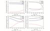 |
Fig. 1 Investment strategies under different loss aversion parameters |
When  (Fig. 1(a)), fund managers invest more money in risky assets in order to obtain the wealth value of 100 at the beginning, since the wealth value of 100 is not a difficult target to reach, fund managers have a relatively moderate aversion to risk at this time. During the wealth accumulation period of 30 years, fund managers do not plan to make significant adjustments to the allocation of funds. With the accumulation of wealth funds in accounts to a certain amount, fund managers will reduce investment in risky assets to avoid losses. Cash short positions gradually decreased from 2.5 to 0.3, and the proportion of risky assets held also decreased correspondingly.
In Fig. 1(b), the loss aversion parameter  , in fact, the wealth value of 1 000 is extremely difficult for fund management to obtain, and fund managers are risk averse at the beginning. In order to pursue more wealth accumulation, fund managers invest more money in risky assets when the wealth value accumulation is small at the beginning. As the accumulation of medium-term account funds meets the need for minimum living guarantee, fund managers will reduce risks and the proportion of risky assets invested becomes smaller. Compared with the risk asset investment ratio of 1.6 at the beginning of the period, the risk asset investment ratio is only about 0.4 at the end of the period, and the holding of cash assets accounts for 0.6.
In Fig. 1(c), when the loss aversion parameter is 10 000, fund managers are completely risk averse, and it is almost impossible for fund managers to achieve a wealth value of 10 000. In the early days of the pension fund, managers invest a lot of wealth in risk assets and choose to hold a certain amount of cash bears. As the wealth has accumulated, stock holdings gradually decreased from 1.8 to 0.2, and the proportion of bonds invested also fell to 0. Compared with the significant reduction in risky assets, risk-free assets are on the rise, increasing from -2 at the beginning to around 0.75 at the end of the period.
In Fig. 1(d), We assume that the replacement rate of pension benefits that pension participants expect to receive after retirement and pre-retirement wages is 0.4, then the investment strategy of fund managers has changed a lot. We can see that, with the accumulation of wealth in pension fund accounts over time, the proportion of fund managers' investment in risky assets is not less before pension participants retire, instead of showing a slow growth trend.
Figure 2 describes the impact of different levels of bequest motivation on investment strategies under the same economic environment. When the bequest motivation level is 100 and the initial wealth accumulation is small (Fig. 2(a)), fund managers are willing to hold rolling bonds of 1, while short-selling cash assets of 0.3 choose to hold stocks of 0.3. As wealth is accumulated enough to satisfy the bequest motivation, fund managers will sold a lot of rolling bonds and opted to hold cash assets, reducing risk. As we can see, at the end of the period, the fund manager held only 0.1 risky assets and 1.9 cash.
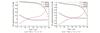 |
Fig. 2 Investment strategies under different bequest motivation |
In Fig. 2(b), the bequest level  is easier to reach than 100. When the bequest level is high, fund managers need more funds to invest in risky assets to obtain a higher level of wealth. So at the start of the session, the manager shorted nearly 0.6 of the position and held 1.6 of the risky assets, accumulating as much wealth as possible. However, because a higher level of bequest motivation is basically difficult to obtain in practice, after meeting the minimum living guarantee of participants, fund managers will gradually reduce risks, sell rolling bonds and stocks, and choose to hold cash.
4 Conclusion
In this paper, under the S-shaped utility function of loss aversion, the introduction of bequest motivations and the substitution rate between receiving pension benefits after retirement and wages before retirement, we set stochastic inflation then use Legendre transformation and martingale method to solve the optimal terminal pension surplus and the optimal investment strategy. Finally, the numerical simulation is used to analyze the impact of different loss aversion parameters and bequest motivations on DC pension investment strategies. Through numerical analysis, it can be concluded that loss-averse investors will invest more in stocks and bonds than in cash, and even hold a certain proportion of cash short in some cases in order to obtain more investment returns in order to obtain more wealth. Constrained by the bequest motivation, fund managers are more willing to increase the proportion of cash assets.
At the same time, after adding the replacement rate between pension benefits and wages, we can see that in order to achieve a certain degree of replacement rate, the investment strategy of pension funds has changed to a certain extent. In the future, we can do some in-depth research under the framework of this article, such as adding random payment rates, introducing random lifespan risks, replacing utility functions and so on. These are also our future research directions.
References
- Boulier J F, Huang S J, Taillard G. Optimal management under stochastic interest rates: the case of a protected defined contribution pension fund [J]. Insurance Mathematics and Economics, 2001, 28(2): 173-189. [Google Scholar]
- Gao J W. Optimal portfolios for DC pension plans under a CEV model [J]. Insurance: Mathematics and Economics, 2009, 44(3): 479-490. [CrossRef] [MathSciNet] [Google Scholar]
- Zhang L, Li D P, Lai Y Z. Equilibrium investment strategy for a defined contribution pension plan under stochastic interest rate and stochastic volatility [J]. Journal of Computational and Applied Mathematics, 2020, 368: 112536. [CrossRef] [MathSciNet] [Google Scholar]
- Tiro K, Basimanebotlhe O, Offen E R. Stochastic analysis on optimal portfolio selection for DC pension plan with stochastic interest and inflation rate[J]. Journal of Mathematical Finance, 2021, 11(4): 579-596. [Google Scholar]
- Wang Y, Xu X, Zhang J Z. Optimal investment strategy for DC pension plan with stochastic income and inflation risk under the Ornstein-Uhlenbeck model [J]. Mathematics, 2021, 9(15): 1756-1771. [CrossRef] [Google Scholar]
- Han N W, Hung M W. Optimal asset allocation for DC pension plans under inflation [J]. Insurance: Mathematics and Economics, 2012, 51(1): 172-181. [Google Scholar]
- Wu H L, Zhang L, Chen H. Nash equilibrium strategies for a defined contribution pension management [J]. Insurance: Mathematics and Economics, 2015, 62: 202-214. [Google Scholar]
- Baltas I, Dopierala L, Kolodziejczyk K, et al. Optimal management of defined contribution pension funds under the effect of inflation, mortality and uncertainty [J]. European Journal of Operational Research, 2022, 298(3): 1162-1174. [CrossRef] [MathSciNet] [Google Scholar]
- Hou L, Yang X T, Li Q. Urban household bequest motive in China: An estimation based on micro household finance data [J]. The Journal of World Economy, 2021, 44(5): 79-104(Ch). [Google Scholar]
- Choi S, Wilmarth M J. The moderating role of depressive symptoms between financial assets and bequests expectation [J]. Journal of Family and Economic Issues, 2019, 40(3): 498-510. [Google Scholar]
- Shi A L, Li Z F. Optimal investment strategy of DC pension plan with bequest motivation and minimum performance constraints [J]. Journal of Systems Science and Mathematical, 2021, 41(7): 1905-1926. [Google Scholar]
- Kahneman D, Tversky A. Prospect theory: An analysis of decision under risk [J]. Econometrica, 1979, 47(2): 263-291. [CrossRef] [Google Scholar]
- Guan G H, Liang Z X. Optimal management of DC pension plan under loss aversion and Value-at-Risk constraints [J]. Insurance: Mathematics and Economics, 2016, 69: 224-237. [Google Scholar]
- Chen Z, Li Z F, Zeng Y, et al. Asset allocation under loss aversion and minimum performance constraint in a DC pension plan with inflation risk [J]. Insurance: Mathematics and Economics, 2017, 75: 137-150. [Google Scholar]
- Wang C Y, Fu C Y, Sheng G X. Optimal investment of DC pension under the inflation and loss aversion [J]. Journal of University of Science and Technology of China, 2018, 48(5): 420-430(Ch). [Google Scholar]
All Figures
|
Fig. 1 Investment strategies under different loss aversion parameters |
| In the text | |
|
Fig. 2 Investment strategies under different bequest motivation |
| In the text | |
Current usage metrics show cumulative count of Article Views (full-text article views including HTML views, PDF and ePub downloads, according to the available data) and Abstracts Views on Vision4Press platform.
Data correspond to usage on the plateform after 2015. The current usage metrics is available 48-96 hours after online publication and is updated daily on week days.
Initial download of the metrics may take a while.