© Wuhan University 2024

0 Introduction

Consider the following equation:

$\{\begin{array}{ll}-\mathrm{\Delta }{u}_i-\frac{h}{{\left|x\right|}^{\mathrm{2}}}{u}_i+V(x)u_i={\lambda }_i(V,h)u_i& \mathrm{i}\mathrm{n}\mathrm{\Omega },\\ u_i=\mathrm{0}& \mathrm{o}\mathrm{n}\partial \mathrm{\Omega },\end{array}$

where $\mathrm{\Omega }\subseteq {\mathbb{R}}^N(N=\mathrm{3})$ is an open and bounded ball with $|\mathrm{\Omega }|=\mathrm{1}$, 0$=(\mathrm{0,0},\mathrm{0})\in \partial \mathrm{\Omega }\in C^{\mathrm{1}}$, and $h\in (\mathrm{0},h_{\mathrm{*}}=\frac{{(N-\mathrm{2})}^{\mathrm{2}}}{\mathrm{4}})$ is a constant, $V$ is the potential function, and $V\in {V}=\{a\in L^{\mathrm{\infty }}(\mathrm{\Omega })|\mathrm{0}\le a\le M\hspace{1em}\mathrm{a}.\mathrm{e}.,M\mathrm{i}\mathrm{s}\mathrm{a}\mathrm{g}\mathrm{i}\mathrm{v}\mathrm{e}\mathrm{n}\mathrm{c}\mathrm{o}\mathrm{n}\mathrm{s}\mathrm{t}\mathrm{a}\mathrm{n}\mathrm{t}\}$.

In the Sobolev space $H_{\mathrm{0}}^{\mathrm{1}}(\mathrm{\Omega })$, its norm is:

${\Vert u\Vert }_{H_{\mathrm{0}}^{\mathrm{1}}(\mathrm{\Omega })}={\left(\sum _{\left|\alpha \right|\le \mathrm{1}}{\int }_{\mathrm{\Omega }}{\left|D^{\alpha }u\right|}^{\mathrm{2}}\mathrm{d}x\right)}^{\frac{\mathrm{1}}{\mathrm{2}}}$

or the equivalent norm: ${\Vert u\Vert }_{H_{\mathrm{0}}^{\mathrm{1}}(\mathrm{\Omega })}={\Vert Du\Vert }_{L^{\mathrm{2}}(\mathrm{\Omega })}$ (by using the Poincaré inequality).

Denote

$\mathrm{\mathscr{H}}=\left\{u\in H_{\mathrm{0}}^{\mathrm{1}}(\mathrm{\Omega })|\frac{\mathrm{1}}{\left|x\right|}u\in L^{\mathrm{2}}(\mathrm{\Omega }),\underset{|x|\to \mathrm{0}}{\mathrm{l}\mathrm{i}\mathrm{m}}{\left|x\right|}^{-\frac{\mathrm{1}}{\mathrm{2}}}u(x)=\mathrm{0}\right\}.$

In quantum mechanics, actually, the eigenvalue problem of operators in the theory of Hilbert space is mentioned by many researchers. In 2013, Tyagi^[1] considered a singular eigenvalue problem involving Hardy's potential with Dirichlet boundary condition and gave that the problem possesses a continuous family of eigenvalues. Gesztesy and Zinchenko^[2] showed the case of self-adjoint half-line Schrödinger operators on $(a,\mathrm{\infty })$ with a potential strongly singular at the endpoint a. Nursultanov ^[3] found that asymptotic formulas for the eigenvalues of the Sturm-Liouville operator on the finite interval, with potentials having a strong negative singular at one endpoint. Haese-Hill ^[4] studied the spectral properties of its complex regularizations of the form:

$L=-\frac{{\mathrm{d}}^{\mathrm{2}}}{\mathrm{d}{x}^{\mathrm{2}}}+m(m+\mathrm{1})w^{\mathrm{2}}f(wx+z_{\mathrm{0}}),z_{\mathrm{0}}\in \mathbb{C},$

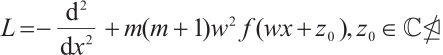
where $w$ is one of the half-periods of $f(z)$ and $f(z)$ is the classical Weierstrass elliptic function. Li and Zhang ^[5] studied the numerical approximation of eigenvalue problems of the Schrödinger operator $-\mathrm{\Delta }u+\frac{x^{\mathrm{2}}}{{\left|x\right|}^{\mathrm{2}}}u$. Homa and Hryniv ^[6] proved analogues of the classical Sturm comparison and oscillation theorems for equations $-(p{u}^{\text{'}}{)}^{\text{'}}+qu=\lambda ru$ on a finite interval with real-valued distributional potentials.

Due to the presence of singular terms such as $-\frac{h}{{\left|x\right|}^{\mathrm{2}}}$ in the differential equation, the properties of the equation differ from those of traditional differential equations, constituting singular differential equations. The existence of this particular term makes it challenging to directly apply the classical Sobolev space framework and its related properties to the analysis of such equations. To effectively handle this singularity, this paper introduces weighted Sobolev spaces. Within this newly constructed framework, the existence, uniqueness, and regularity of solutions to singular differential equations are successfully established. The establishment of these properties not only deepens our understanding of solutions to singular differential equations but also lays a solid foundation for further research and applications.

Additionally, a comprehensive description of spectral theory for singular differential equations is provided within this new framework. The characteristics of the equation's eigenvalues and eigenfunctions can be more accurately characterized by introducing weighted Sobolev spaces. This theory holds profound mathematical significance and offers new perspectives and methods for solving practical problems.

1 Preliminary

Lemma 1   The space $(\mathrm{\mathscr{H}},\Vert \cdot {\Vert }_{H^{\mathrm{1}}})$ is a Hilbert space.

Proof   Let $\{u_n{\}}_{n\in \mathbb{N}}\subset \mathrm{\mathscr{H}}$ is a Cauchy sequence. Note that $\mathrm{\mathscr{H}}\subset H_{\mathrm{0}}^{\mathrm{1}}(\mathrm{\Omega })$, then there exists $u^{\mathrm{*}}\in H_{\mathrm{0}}^{\mathrm{1}}(\mathrm{\Omega })$ such that $u_n\to u^{\mathrm{*}}$ strongly in $H_{\mathrm{0}}^{\mathrm{1}}$.

By using the Sobolev Embedding Theorem, we have $u_n\to u^{\mathrm{*}}$ strongly in $L^q(\mathrm{\Omega })$ for $N=\mathrm{3}$.

By using the Hardy-Sobolev inequality ^[7]:

${\int }_{\mathrm{\Omega }}{\left|Du\right|}^p\mathrm{d}x\ge {(\frac{n-p}{p})}^p{\int }_{\mathrm{\Omega }}\frac{|u(x){|}^p}{{\left|x\right|}^p}\mathrm{d}x$ holds for $u\in W_{\mathrm{0}}^{\mathrm{1},p}(\mathrm{\Omega })$,

where $W_{\mathrm{0}}^{\mathrm{1},p}(\mathrm{\Omega })$ is the completion of $C_{\mathrm{0}}^{\mathrm{\infty }}(\mathrm{\Omega })$ in the norm:

${\Vert u\Vert }_{\mathrm{1},p,\mathrm{\Omega }}:={\left({\int }_{\mathrm{\Omega }}{\left|u(x)\right|}^p\mathrm{d}x+{\int }_{\mathrm{\Omega }}{\left|Du\right|}^p\mathrm{d}x\right)}^{\frac{\mathrm{1}}{p}}.$

We have:

${\int }_{\mathrm{\Omega }}{\left|Du\right|}^{\mathrm{2}}\mathrm{d}x\ge {(\frac{\mathrm{3}-\mathrm{2}}{\mathrm{2}})}^{\mathrm{2}}{\int }_{\mathrm{\Omega }}\frac{u{(x)}^{\mathrm{2}}}{{\left|x\right|}^{\mathrm{2}}}\mathrm{d}x=\frac{\mathrm{1}}{\mathrm{4}}{\int }_{\mathrm{\Omega }}\frac{u{(x)}^{\mathrm{2}}}{{\left|x\right|}^{\mathrm{2}}}\mathrm{d}x,$

${\int }_{\mathrm{\Omega }}\frac{u{(x)}^{\mathrm{2}}}{{\left|x\right|}^{\mathrm{2}}}\mathrm{d}x\le \mathrm{4}{\int }_{\mathrm{\Omega }}{\left|Du\right|}^{\mathrm{2}}\mathrm{d}x$

which means that

$\Vert \frac{u}{\left|x\right|}{\Vert }_{L^{\mathrm{2}}}\le {\Vert Du\Vert }_{L^{\mathrm{2}}}$(1)

So, we have $\{u_n{\}}_{n\in \mathbb{N}}\subset \mathrm{\mathscr{H}}$, and

$\Vert \frac{\mathrm{1}}{\left|x\right|}{u}_n-\frac{\mathrm{1}}{\left|x\right|}{u}_m{\Vert }_{L^{\mathrm{2}}}\le C{\Vert u_n-u_m\Vert }_{H_{\mathrm{0}}^{\mathrm{1}}}\to \mathrm{0},\hspace{1em}n,m\to \mathrm{\infty }$

Then, there exists $v^{\mathrm{*}}\in L^{\mathrm{2}}(\mathrm{\Omega })$ such that

$\frac{\mathrm{1}}{\left|x\right|}{u}_n\to v^{\mathrm{*}}$ strongly in $L^{\mathrm{2}}(\mathrm{\Omega })$

and

$\begin{array}{l}{\int }_{\mathrm{\Omega }}{\left|u_n-v^{\mathrm{*}}\left|x\right|\right|}^{\mathrm{2}}\mathrm{d}x={\int }_{\Omega }|x{|}^{\mathrm{2}}{\left|\frac{\mathrm{1}}{\left|x\right|}{u}_n-v^{\mathrm{*}}\right|}^{\mathrm{2}}\mathrm{d}x\\ \le {\int }_{\mathrm{\Omega }}{\left|\frac{\mathrm{1}}{\left|x\right|}{u}_n-v^{\mathrm{*}}\right|}^{\mathrm{2}}\mathrm{d}x\to \mathrm{0},\mathrm{a}\mathrm{s}n\to \mathrm{\infty },\end{array}$

which shows that $u_n\to v^{\mathrm{*}}\left|x\right|$ strongly in $L^{\mathrm{2}}(\mathrm{\Omega })$. From the assumptions $v^{\mathrm{*}}\left|x\right|=u^{\mathrm{*}}$ in $L^{\mathrm{2}}(\mathrm{\Omega })$, then $\frac{\mathrm{1}}{\left|x\right|}{u}_n=v^{\mathrm{*}}\in L^{\mathrm{2}}(\mathrm{\Omega })$.

Denote

$L:=-\mathrm{\Delta }-\frac{\mathrm{1}}{\left|x\right|}+V(x)$(2)

In the sense of distribution, for $g\in L^{\mathrm{2}}(\mathrm{\Omega })$, $u\in \mathrm{\mathscr{H}}$ is a solution of the following equation

$\{\begin{array}{ll}Lu=g,& \mathrm{i}\mathrm{n}\mathrm{\Omega };\\ u=\mathrm{0},& \mathrm{o}\mathrm{n}\partial \mathrm{\Omega },\end{array}$(3)

which is equivalent to the following equality:

${\int }_{\mathrm{\Omega }}g\phi (x)\mathrm{d}x={\int }_{\mathrm{\Omega }}Lu(x)\phi (x)\mathrm{d}x,\hspace{1em}\forall \phi (x)\in C_c^{\mathrm{\infty }}(\mathrm{\Omega })$

Definition 1   (i) The bilinear form $B(\cdot ,\cdot )$ associated with the elliptic operator $L$ defined by (2) is

$B(u,v)={\int }_{\mathrm{\Omega }}\left(Du\cdot Dv-\frac{h}{{\left|x\right|}^{\mathrm{2}}}u\cdot v+Vu\cdot v\right)\mathrm{d}x,\hspace{1em}\forall u,v\in \mathrm{\mathscr{H}}$

(ii) We say that $u\in \mathrm{\mathscr{H}}$ is a weak solution of the boundary-value problem (3) if

$B(u,v)={(g,v)}_{L^{\mathrm{2}}(\mathrm{\Omega })}$

For all $v\in \mathrm{\mathscr{H}}$, where $(\cdot ,\cdot )$ denotes the inner product in $L^{\mathrm{2}}(\mathrm{\Omega })$.

Theorem 1   Let $B:\mathrm{\mathscr{H}}\times \mathrm{\mathscr{H}}\to \mathbb{R}$ be defined as above. Then, there exist constants $C>\mathrm{0}$ such that

$|B(u,v)|\le C{\Vert u\Vert }_{H^{\mathrm{1}}}{\Vert v\Vert }_{H^{\mathrm{1}}}$

and

$C{\Vert u\Vert }_{H^{\mathrm{1}}}^{\mathrm{2}}\le B(u,u)$(4)

for all $u,v\in H_{\mathrm{0}}^{\mathrm{1}}(\mathrm{\Omega })$.

Proof   We readily check that:

$\begin{array}{l}|B(u,v)|=\left|{\int }_{\Omega }(Du\cdot Dv-\frac{h}{{\left|x\right|}^{\mathrm{2}}}u\cdot v+V(x)u\cdot v)\mathrm{d}x\right|\\ \le {\int }_{\Omega }|Du\cdot Dv|\mathrm{d}x+h{\int }_{\Omega }|\frac{u}{\left|x\right|}||\frac{v}{\left|x\right|}|\mathrm{d}x+{\int }_{\Omega }|V(x)u\cdot v|\mathrm{d}x\\ \le {\Vert Du\Vert }_{L^{\mathrm{2}}}{\Vert Dv\Vert }_{L^{\mathrm{2}}}+h{\Vert \frac{\mathrm{1}}{\left|x\right|}u\Vert }_{L^{\mathrm{2}}}{\Vert \frac{\mathrm{1}}{\left|x\right|}v\Vert }_{L^{\mathrm{2}}}+M{\Vert u\Vert }_{L^{\mathrm{2}}}{\Vert v\Vert }_{L^{\mathrm{2}}}\end{array}$

for all $u,v\in H_{\mathrm{0}}^{\mathrm{1}}(\mathrm{\Omega })$ by Cauchy-Schwarz inequality.

Then we have

$\begin{array}{l}\left|B(u,v)\right|\le {\Vert Du\Vert }_{L^{\mathrm{2}}}{\Vert Dv\Vert }_{L^{\mathrm{2}}}+C{\Vert Du\Vert }_{L^{\mathrm{2}}}{\Vert Dv\Vert }_{L^{\mathrm{2}}}\\ +C{\Vert Du\Vert }_{L^{\mathrm{2}}}{\Vert Dv\Vert }_{L^{\mathrm{2}}}\\ \le C{\Vert Du\Vert }_{L^{\mathrm{2}}}{\Vert Dv\Vert }_{L^{\mathrm{2}}}\end{array}$

by Lemma 1 and Poincaré inequality.

What's more, since $V(x)\ge \mathrm{0}$ a.e., we can obtain that

$\begin{array}{l}B(u,u)={\int }_{\mathrm{\Omega }}\left({\left|Du\right|}^{\mathrm{2}}-\frac{h}{{\left|x\right|}^{\mathrm{2}}}{u}^{\mathrm{2}}+V{u}^{\mathrm{2}}\right)\mathrm{d}x\\ \ge {\int }_{\mathrm{\Omega }}{\left|Du\right|}^{\mathrm{2}}\mathrm{d}x-h{\int }_{\mathrm{\Omega }}\frac{u^{\mathrm{2}}}{{\left|x\right|}^{\mathrm{2}}}\mathrm{d}x\\ \ge {{\int }_{\mathrm{\Omega }}\left|Du\right|}^{\mathrm{2}}\mathrm{d}x-\mathrm{4}h{\Vert Du\Vert }_{L^{\mathrm{2}}}^{\mathrm{2}}\\ =(\mathrm{1}-\mathrm{4}h){\Vert Du\Vert }_{L^{\mathrm{2}}}^{\mathrm{2}}\\ =C{\Vert Du\Vert }_{L^{\mathrm{2}}}^{\mathrm{2}}=C{\Vert u\Vert }_{H^{\mathrm{1}}}^{\mathrm{2}}.\end{array}$

Corollary 1   Let $g\in L^{\mathrm{2}}(\mathrm{\Omega })$ be a given function, then the elliptic equation $Lu=g$, $u\in \mathrm{\mathscr{H}}$ has a unique weak solution.

Proof   By Theorem 1 and Lax-Milgram theorem, we can conclude the corollary.

Corollary 2   The operator $L:\mathrm{\mathscr{H}}\to {\mathrm{\mathscr{H}}}^{\text{'}}$ is a continuous, coercive, surjective, and linear operator, where $H^{\text{'}}$ is the dual space of $\mathrm{\mathscr{H}}$.

Proof   It is evident that $L$ is a linear operator.

${\Vert Lu\Vert }_{{\mathrm{\mathscr{H}}}^{\text{'}}}=\underset{v\in \mathrm{\mathscr{H}},{\Vert v\Vert }_{H_{\mathrm{0}}^{\mathrm{1}}}=\mathrm{1}}{\mathrm{s}\mathrm{u}\mathrm{p}}<Lu,v{>}_{{\mathrm{\mathscr{H}}}^{\text{'}},\mathrm{\mathscr{H}}}\ge <Lu,\frac{u}{\Vert u\Vert }{>}_{{\mathrm{\mathscr{H}}}^{\text{'}},\mathrm{\mathscr{H}}}$

$\ge \frac{C<u,u{>}_{\mathrm{\mathscr{H}}}}{{\Vert u\Vert }_{H^{\mathrm{1}}}}=C{\Vert u\Vert }_{H^{\mathrm{1}}}$

$\begin{array}{l}{\Vert Lu\Vert }_{{\mathrm{\mathscr{H}}}^{\text{'}}}=\underset{v\in \mathrm{\mathscr{H}},{\Vert v\Vert }_{H_{\mathrm{0}}^{\mathrm{1}}}=\mathrm{1}}{\mathrm{s}\mathrm{u}\mathrm{p}}<Lu,v{>}_{{\mathrm{\mathscr{H}}}^{\text{'}},\mathrm{\mathscr{H}}}\\ =\underset{v\in \mathrm{\mathscr{H}},{\Vert v\Vert }_{H_{\mathrm{0}}^{\mathrm{1}}}=\mathrm{1}}{\mathrm{s}\mathrm{u}\mathrm{p}}{\int }_{\mathrm{\Omega }}\left(Du\cdot Dv-\frac{h}{{\left|x\right|}^{\mathrm{2}}}u\cdot v+V(x)u\cdot v\right)\mathrm{d}x\\ =\underset{v\in \mathrm{\mathscr{H}},{\Vert v\Vert }_{H_{\mathrm{0}}^{\mathrm{1}}}=\mathrm{1}}{\mathrm{s}\mathrm{u}\mathrm{p}}B(u,v)\le C{\Vert u\Vert }_{H_{\mathrm{0}}^{\mathrm{1}}}.\end{array}$

Let $g\in {\mathrm{\mathscr{H}}}^{\text{'}}$, by using the Lax-Milgram theorem^[8], we can see that there exists a unique element $u\in \mathrm{\mathscr{H}}$ such that

$<Lu,v{>}_{{\mathrm{\mathscr{H}}}^{\text{'}},\mathrm{\mathscr{H}}}=B(u,v)=<g,v{>}_{{\mathrm{\mathscr{H}}}^{\text{'}},\mathrm{\mathscr{H}}},\hspace{1em}\forall v\in \mathrm{\mathscr{H}}$

Note that $C_c^{\mathrm{\infty }}(\mathrm{\Omega })\subset \mathrm{\mathscr{H}}$, thus

$Lu=g$

in the sense of distribution.

Consequently, $L:\mathrm{\mathscr{H}}\to {\mathrm{\mathscr{H}}}^{\text{'}}$ is a continuous, coercive, surjective, and linear operator.

Lemma 2   Assume $g\in L^{\mathrm{2}}(\mathrm{\Omega })$, let u be a weak solution to the equation

$Lu=g,u\in \mathrm{\mathscr{H}}.$(5)

Then $u\in H_{\mathrm{l}\mathrm{o}\mathrm{c}}^{\mathrm{2}}(\mathrm{\Omega })$. Moreover,

${\Vert u\Vert }_{H^{\mathrm{2}}({\mathrm{\Omega }}^{″})}\le C\left({\Vert g\Vert }_{L^{\mathrm{2}}}+{\sigma }^{-\mathrm{1}}{\Vert u\Vert }_{H^{\text{'}}}\right),\hspace{1em}\forall \sigma \in (\mathrm{0,1})$(6)

where ${\mathrm{\Omega }}^{″}=\mathrm{\Omega }\backslash B(\mathrm{0},\sigma )$.

Proof   (1) For all $x\in \mathrm{\Omega }$, let $s_{\mathrm{0}}>\mathrm{0}$ be small such that $\mathrm{d}\mathrm{i}\mathrm{s}\mathrm{t}(x,\partial \mathrm{\Omega })>\mathrm{2}{s}_{\mathrm{0}}$. We take

${\mathrm{\Omega }}^{\text{'}}=\{x|x\in \mathrm{\Omega },\mathrm{d}\mathrm{i}\mathrm{s}\mathrm{t}(x,\partial \mathrm{\Omega })>\mathrm{2}{s}_{\mathrm{0}}\}$

Select a smooth function $\zeta$ satisfying

$\zeta \equiv \mathrm{1}\mathrm{o}\mathrm{n}{\mathrm{\Omega }}^{\text{'}}\mathrm{a}\mathrm{n}\mathrm{d}\zeta \equiv \mathrm{0}\mathrm{o}\mathrm{n}\mathrm{\Omega }\backslash {\mathrm{\Omega }}^{\text{'}},\hspace{1em}\mathrm{0}\le \zeta \le \mathrm{1}$

Since $u$ is a weak solution of (5), we have $B(u,v)=(g,v)$ for all $v\in \mathrm{\mathscr{H}}$. Then

${\int }_{\mathrm{\Omega }}Du\cdot Dv\mathrm{d}x={\int }_{\mathrm{\Omega }}\left(gv+\frac{h}{{\left|x\right|}^{\mathrm{2}}}uv-Vuv\right)\mathrm{d}x={\int }_{\mathrm{\Omega }}\tilde{g}v\mathrm{d}x$

where $\tilde{g}=g+\frac{h}{{\left|x\right|}^{\mathrm{2}}}u-Vu$.

Set

$D^{h}u(x)=\frac{u(x+s)-u(x)}{s},\hspace{1em}|s|\le s_{\mathrm{0}},s\ne \mathrm{0}$

$v=D^{-s}{\zeta }^{\mathrm{2}}{D}^{s}u$

Then, on the one hand, by the Cauchy equality with weight and difference quotient estimate, we have

$\begin{array}{l}{\int }_{\mathrm{\Omega }}Du\cdot Dv\mathrm{d}x=-{\int }_{\mathrm{\Omega }}Du\cdot D(D^{-s}{\zeta }^{\mathrm{2}}{D}^{s}u)\mathrm{d}x\\ ={\int }_{\Omega }(D^s(Du))(D({\zeta }^{\mathrm{2}}{D}^{s}u))\mathrm{d}x\\ ={\int }_{\Omega }(D^s(Du))(\mathrm{2}\zeta D\zeta D^{s}u)\mathrm{d}x+{\int }_{\Omega }(D^s(Du)){\zeta }^{\mathrm{2}}(D^s(Du))\mathrm{d}x\end{array}$

$\begin{array}{l}\ge \frac{\mathrm{1}}{\mathrm{2}}{\int }_{\mathrm{\Omega }}{\zeta }^{\mathrm{2}}|D^s(Du){|}^{\mathrm{2}}\mathrm{d}x-C{\int }_{\Omega }|D^{s}u{|}^{\mathrm{2}}\mathrm{d}x\\ \ge \frac{\mathrm{1}}{\mathrm{2}}{\int }_{\mathrm{\Omega }}{\zeta }^{\mathrm{2}}|D^s(Du){|}^{\mathrm{2}}\mathrm{d}x-C{\int }_{\Omega }|Du{|}^{\mathrm{2}}\mathrm{d}x.\end{array}$

On the other hand, by difference quotient estimate, we have

$\begin{array}{l}{\int }_{\mathrm{\Omega }}{\left|v\right|}^{\mathrm{2}}\mathrm{d}x={{\int }_{\mathrm{\Omega }}\left|D^{-s}({\zeta }^{\mathrm{2}}{D}^{s}u)\right|}^{\mathrm{2}}\mathrm{d}x\\ \le C{\int }_{\mathrm{\Omega }}{\left|D({\zeta }^{\mathrm{2}}{D}^{s}u)\right|}^{\mathrm{2}}\mathrm{d}x\le C{\int }_{\Omega }({\left|Du\right|}^{\mathrm{2}}+{\zeta }^{\mathrm{2}}{\left|D^s(Du)\right|}^{\mathrm{2}})\mathrm{d}x.\end{array}$

Thus, the Cauchy inequality with weight implies

$\left|{\int }_{\mathrm{\Omega }}\tilde{g}v\mathrm{d}x\right|\le \frac{\mathrm{1}}{\mathrm{4}}{\int }_{\mathrm{\Omega }}{\zeta }^{\mathrm{2}}{\left|D^s(Du)\right|}^{\mathrm{2}}\mathrm{d}x+C{\int }_{\mathrm{\Omega }}{g}^{\mathrm{2}}+u^{\mathrm{2}}+{\left|Du\right|}^{\mathrm{2}}\mathrm{d}x$

where $C$ is depend on $\frac{\mathrm{1}}{s_{\mathrm{0}}^{\mathrm{2}}}$.

Consequently,

${{\int }_{{\mathrm{\Omega }}^{\text{'}}}\left|D^s(Du)\right|}^{\mathrm{2}}\mathrm{d}x\le C{\int }_{\mathrm{\Omega }}\left(g^{\mathrm{2}}+u^{\mathrm{2}}+{\left|Du\right|}^{\mathrm{2}}\right)\mathrm{d}x,\hspace{1em}\forall \left|s\right|\le \left|s_{\mathrm{0}}\right|$

From the difference quotient, we deduce $Du\in H_{\mathrm{l}\mathrm{o}\mathrm{c}}^{\mathrm{1}}(\mathrm{\Omega })$ and thus $u\in H_{\mathrm{l}\mathrm{o}\mathrm{c}}^{\mathrm{2}}(\mathrm{\Omega })$.

(2) For any $\sigma \in (\mathrm{0,1})$, according to (5)

$\left|\mathrm{\Delta }u\right|\le \left|\frac{h}{\left|x^{\mathrm{2}}\right|}u-Vu+gu\right|\le h|\frac{u}{{\left|x\right|}^{\mathrm{2}}}|+\left|Vu\right|+\left|gu\right|,\forall x\in {\mathrm{\Omega }}^{″}$

From which, Cauchy-Schwarz inequality and (1), we deduce that:

$\begin{array}{l}{{\int }_{{\mathrm{\Omega }}^{″}}\left|\mathrm{\Delta }u\right|}^{\mathrm{2}}\mathrm{d}x\le C\left({\int }_{{\Omega }^{″}}|\frac{h}{{\left|x\right|}^{\mathrm{2}}}u{|}^{\mathrm{2}}\mathrm{d}x+{\int }_{{\mathrm{\Omega }}^{″}}{\left|Vu\right|}^{\mathrm{2}}\mathrm{d}x+{{\int }_{{\mathrm{\Omega }}^{″}}\left|g\right|}^{\mathrm{2}}\mathrm{d}x\right)\\ \le C\left(\frac{\mathrm{1}}{{\sigma }^{\mathrm{2}}}{{\int }_{\mathrm{\Omega }}\left|Du\right|}^{\mathrm{2}}\mathrm{d}x+{{\int }_{\mathrm{\Omega }}\left|u\right|}^{\mathrm{2}}\mathrm{d}x+{\Vert g\Vert }_{L^{\mathrm{2}}}\right)\\ \le C\left(\frac{\mathrm{1}}{{\sigma }^{\mathrm{2}}}{\Vert Du\Vert }_{L^{\mathrm{2}}}+{\Vert u\Vert }_{L^{\mathrm{2}}}+{\Vert g\Vert }_{L^{\mathrm{2}}}\right)\\ \le C\left(\frac{\mathrm{1}}{\sigma }{\Vert u\Vert }_{H^{\mathrm{1}}}+{\Vert g\Vert }_{L^{\mathrm{2}}}\right),\end{array}$

where we used Poincaré inequality in the equality, consequently, (6) holds.

Remark 1   Under the assumptions of the Lemma 2, (i) It seems that $u\notin H^{\mathrm{2}}(\mathrm{\Omega })$ since $L$ is singular at $x=\mathrm{0}$; (ii) From the Sobolev Embedding Theorem, it is clear that $u\in C^{\mathrm{1},\frac{\mathrm{1}}{\mathrm{2}}}({\mathrm{\Omega }}^{″})$.

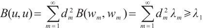
Proposition 1   Let $\sigma (L)$ denotes the spectrum of L. Then $\sigma (L)\subset \mathbb{R}$ and $\sigma (L)$ is at most countable. Let $\sigma (L)=\{{\lambda }_k{\}}_{k=\mathrm{1}}^{\mathrm{\infty }}$, where the eigenvalue is counted according to its multiplicity, then

$\mathrm{0}<{\lambda }_{\mathrm{1}}\le {\lambda }_{\mathrm{2}}\le \cdots ,and{\lambda }_k\to \mathrm{\infty }ask\to \mathrm{\infty }.$

Finally, there exists an orthonormal basis $\{w_k{\}}_{k=\mathrm{1}}^{\mathrm{\infty }}$ of $L^{\mathrm{2}}(\mathrm{\Omega })$, where $w_k\in \mathrm{\mathscr{H}}$ is an eigenfunction corresponding to ${\lambda }_k$, that is

$L{w}_k={\lambda }_k{w}_k,\hspace{1em}{w}_k\in \mathrm{\mathscr{H}}.$

Proof   Since $L$ is a coercive, surjective, linear operator, set $T=L^{-\mathrm{1}}$. From the Sobolev Compact Embedding theorem, we deduce that $T:L^{\mathrm{2}}(\mathrm{\Omega })\to L^{\mathrm{2}}(\mathrm{\Omega })$ is a bounded, linear, compact operator. Hence $\sigma (T)$, the spectrum of $T$, is at most countable and has $\mathrm{0}$ as the unique limit point.

For any $g,f\in L^{\mathrm{2}}(\mathrm{\Omega })$, denote $u=Tg$, $v=Tf$, then

$Lu=g,u\in \mathrm{\mathscr{H}};Lv=f,v\in \mathrm{\mathscr{H}}.$

Thus,

$\begin{array}{l}{(Tg,f)}_{L^{\mathrm{2}}}={(u,Lv)}_{L^{\mathrm{2}}}\\ ={\int }_{\mathrm{\Omega }}\left(Du\cdot Dv-\frac{h}{{\left|x\right|}^{\mathrm{2}}}u\cdot v+V(x)u\cdot v\right)\mathrm{d}x\\ ={(Lu,v)}_{L^{\mathrm{2}}}={(g,Tf)}_{L^{\mathrm{2}}},\end{array}$

which shows that $T$ is a symmetric operator.

So, we say that $T$ is a self-adjoint linear operator. And we thereby obtain the assertion of the Proposition by the Standard Functional Analysis 8 ^[8].

Lemma 3   Let $u_i\in \mathrm{\mathscr{H}}$ be the i-th eigenfunction with respect to the eigenfunction ${\lambda }_i$ of $L$ with the potential $V\in {V}$. Then,

${\lambda }_{\mathrm{1}}(V)=\underset{u\in \mathrm{\mathscr{H}},u\ne \mathrm{0}}{\mathrm{m}\mathrm{i}\mathrm{n}}\frac{B(u,u)}{{\Vert u\Vert }_{L^{\mathrm{2}}}^{\mathrm{2}}}$(7)

${\lambda }_{\mathrm{2}}(V)=\underset{u\in E_{\mathrm{1}}^{\perp },u\ne \mathrm{0}}{\mathrm{m}\mathrm{i}\mathrm{n}}\frac{B(u,u)}{{\Vert u\Vert }_{L^{\mathrm{2}}}^{\mathrm{2}}}$(8)

where,

$E_{\mathrm{1}}=\{u\in \mathrm{\mathscr{H}}|(u,u_{\mathrm{1}}{)}_{L^{\mathrm{2}}}=\mathrm{0}\}$

Proof   (i) Let $\sigma (L)=\{{\lambda }_m{\}}_{m=\mathrm{1}}^{\mathrm{\infty }}$ and $\{w_m{\}}_{m=\mathrm{1}}^{\mathrm{\infty }}$ be defined as in Proposition 1. Then

$B(w_m,w_m)={\lambda }_m(w_m,w_m)={\lambda }_m$

and

$B(w_m,w_n)={\lambda }_m(w_m,w_n)=\mathrm{0},\hspace{1em}\forall m,n\in \mathbb{N},m\ne n.$

We observe that $\{{\lambda }_m^{-\frac{\mathrm{1}}{\mathrm{2}}}{w}_m{\}}_{m=\mathrm{1}}^{\mathrm{\infty }}$ is an orthonormal subset of $\mathrm{\mathscr{H}}$ under the new inner product $B(\cdot ,\cdot )$. In fact, according to Theorem 1, Lemma 1, and the Poincaré inequality, we deduce that

$\begin{array}{l}C{\Vert u\Vert }_{H^{\mathrm{1}}}^{\mathrm{2}}\le B(u,u)={\int }_{\Omega }({\left|Du\right|}^{\mathrm{2}}-{\frac{h}{\left|x\right|}}^{\mathrm{2}}{u}^{\mathrm{2}}+V{u}^{\mathrm{2}})\mathrm{d}x\\ \le C{\Vert Du\Vert }_{L^{\mathrm{2}}}^{\mathrm{2}}=C{\Vert u\Vert }_{H^{\mathrm{1}}}^{\mathrm{2}},\end{array}$

i.e., these two norms ${\Vert \cdot \Vert }_{H^{\mathrm{1}}}$ and $\sqrt[]{B(\cdot ,\cdot )}$ are equivalent on $\mathrm{\mathscr{H}}$.

For arbitrary $u\in \mathrm{\mathscr{H}}$ with $B(w_m,u)=\mathrm{0}$, $\forall m\in \mathbb{N}$, it follows that $u={\displaystyle \sum _{m=\mathrm{1}}^{\mathrm{\infty }}}{d}_m{w}_m$ since $\{w_m{\}}_{m=\mathrm{1}}^{\mathrm{\infty }}$ is an orthonormal basis of $L^{\mathrm{2}}(\mathrm{\Omega })$. Therefore

$\mathrm{0}=B(w_m,u)=d_m{\lambda }_m,\hspace{1em}\forall m\in \mathbb{N}.$

We obtain $d_m=\mathrm{0}$, $\forall m\in \mathbb{N}$. Hence $u=\mathrm{0}$.

Finally, we have ${\left\{{\lambda }_m^{-\frac{\mathrm{1}}{\mathrm{2}}}{w}_m\right\}}_{m=\mathrm{1}}^{\mathrm{\infty }}$ is an orthonormal subset of $\mathrm{\mathscr{H}}$ under the new inner product $B(\cdot ,\cdot )$.

(ii) Let $\mathit{u}\in \mathcal{H}$ with ${\Vert \mathit{u}\Vert }_{{\mathit{L}}^{\mathrm{2}}}=\mathrm{1}$. Assume that ${\displaystyle \sum _{\mathit{m}=\mathrm{1}}^{\mathbf{\infty }}}{\mathit{d}}_{\mathit{m}}^{\mathrm{2}}=\mathrm{1}$. We conclude that

$B(u,u)={\displaystyle \sum _{m=\mathrm{1}}^{\mathrm{\infty }}}{d}_m^{\mathrm{2}}B(w_m,w_m)={\displaystyle \sum _{m=\mathrm{1}}^{\mathrm{\infty }}}{d}_m^{\mathrm{2}}{\lambda }_m\ge {\lambda }_{\mathrm{1}}$

according to (i), this proves (7).

(iii) Suppose we have obtained $u_{\mathrm{1}}$, for any $u\perp u_{\mathrm{1}}$, with ${\Vert u\Vert }_{L^{\mathrm{2}}(\mathrm{\Omega })}=\mathrm{1}$, then $u={\displaystyle \sum _{i=\mathrm{2}}^{\infty }}(u,w_i)w_i={\displaystyle \sum _{i=\mathrm{2}}^{\mathrm{\infty }}}{d}_i{w}_i$ and ${\displaystyle \sum _{i=\mathrm{2}}^{\mathrm{\infty }}}{d}_i^{\mathrm{2}}=\mathrm{1}$. Moreover,

$B(u,u)={\displaystyle \sum _{i=\mathrm{2}}^{\mathrm{\infty }}}B(w_i,w_i)={\displaystyle \sum _{i=\mathrm{2}}^{\mathrm{\infty }}}{d}_i^{\mathrm{2}}{\lambda }_i\ge {\lambda }_{\mathrm{2}}$

which implies that $\underset{u\in E_{\mathrm{1}}^{\perp },u\ne \mathrm{0}}{\mathrm{m}\mathrm{i}\mathrm{n}}\frac{B(u,u)}{{\Vert u\Vert }_{L^{\mathrm{2}}}^{\mathrm{2}}}\ge {\lambda }_{\mathrm{2}}.$

By (i), we have $B(w_{\mathrm{2}},w_{\mathrm{2}})={\lambda }_{\mathrm{2}}$, then the result (8) is obtained.

2 Main Results

Theorem 2   There exists $V^{\mathrm{*}}$, $V_{\mathrm{1}}^{\mathrm{*}}$, $V_{\mathrm{2}}^{\mathrm{*}}\in {V}$, such that

${\lambda }_{\mathrm{1}}(V_{\mathrm{1}}^{\mathrm{*}})=\underset{v\in {V}}{\mathrm{i}\mathrm{n}\mathrm{f}}{\lambda }_{\mathrm{1}}(V),\hspace{1em}{\lambda }_{\mathrm{2}}(V_{\mathrm{2}}^{\mathrm{*}})=\underset{v\in {V}}{\mathrm{i}\mathrm{n}\mathrm{f}}{\lambda }_{\mathrm{2}}(V)$

and

$\mathrm{\Gamma }(V^{\mathrm{*}})=\underset{V\in {V}}{\mathrm{i}\mathrm{n}\mathrm{f}}\mathrm{\Gamma }(V)$

where $\mathrm{\Gamma }(V)={\lambda }_{\mathrm{2}}(V)-{\lambda }_{\mathrm{1}}(V)$ is called the fundamental gap with potential $V\in {V}$.

Proof   we will show the proof by the following steps.

Step 1: $\underset{V\in {V}}{\mathrm{i}\mathrm{n}\mathrm{f}}{\lambda }_{\mathrm{1}}(V)$, $\underset{V\in {V}}{\mathrm{i}\mathrm{n}\mathrm{f}}{\lambda }_{\mathrm{2}}(V)$ exists.

For arbitrary $V_{\mathrm{0}}\in {V}$, we have $\underset{V\in {V}}{\mathrm{i}\mathrm{n}\mathrm{f}}{\lambda }_{\mathrm{1}}(V)\le {\lambda }_{\mathrm{1}}(V_{\mathrm{0}})$. Let $\{{V_n}^{\mathrm{\text{'}}}{\}}_{n\in \mathbb{N}}\subset {V}$ be such that

${\lambda }_{\mathrm{1}}(V_n^{\mathrm{1}})\downarrow \underset{V\in {V}}{\mathrm{i}\mathrm{n}\mathrm{f}}{\lambda }_{\mathrm{1}}(V)={\lambda }_{\mathrm{1}}^{\mathrm{*}},\hspace{1em}{\lambda }_{\mathrm{1}}(V_n^{\mathrm{1}})\le {\lambda }_{\mathrm{1}}(V_{\mathrm{0}}),\hspace{1em}\forall n\in \mathbb{N}$

Then there exists a subsequence of $\{V_n^{\mathrm{1}}{\}}_{n\in \mathbb{N}}$, still denoted by itself, and $V_{\mathrm{1}}^{\mathrm{*}}\in {V}$, such that $V_n^{\mathrm{1}}\to V_{\mathrm{1}}^{\mathrm{*}}$ weakly star in $L^{\mathrm{\infty }}(\mathrm{\Omega })$.

Denote $u_n^{\mathrm{1}}$ be the normalized first eigenfunction of $V_n^{\mathrm{1}}$, which means that ${\Vert u_n^{\mathrm{1}}\Vert }_{L^{\mathrm{2}}}=\mathrm{1}$. From (4), we see

$C{\Vert u_n^{\mathrm{1}}\Vert }_{H^{\mathrm{1}}}\le B(u_n^{\mathrm{1}},u_n^{\mathrm{1}})={\lambda }_{\mathrm{1}}(V_n^{\mathrm{1}})\le C,$

where ${\lambda }_{\mathrm{1}}(V_n^{\mathrm{1}})$ is the first eigenvalue of $L$ with the potential $V_n^{\mathrm{1}}$. Thus, there exists a subsequence of $\{u_n^{\mathrm{1}}{\}}_{n\in \mathbb{N}}$, still denoted by itself, and $u_{\mathrm{1}}^{\mathrm{*}}\in \mathrm{\mathscr{H}}$ such that

$u_n^{\mathrm{1}}\to u_{\mathrm{1}}^{\mathrm{*}}weaklyin\mathrm{\mathscr{H}}$(9)

By $\mathrm{\mathscr{H}}\in H_{\mathrm{0}}^{\mathrm{1}}(\mathrm{\Omega })$ and Sobolev Embedding theorem, we deduce that

$u_n^{\mathrm{1}}\to u_{\mathrm{1}}^{\mathrm{*}}\mathrm{s}\mathrm{t}\mathrm{r}\mathrm{o}\mathrm{n}\mathrm{g}\mathrm{l}\mathrm{y}\mathrm{i}\mathrm{n}{L}^{\mathrm{2}}(\mathrm{\Omega }),$(10)

which implies that;

$\Vert u_{\mathrm{1}}^{\mathrm{*}}{\Vert }_{L^{\mathrm{2}}}=\mathrm{1}$(11)

In view of Lemma 1, we have

${\Vert \frac{u_n^{\mathrm{1}}}{\left|x\right|}\Vert }_{L^{\mathrm{2}}}\le C{\Vert {u_n^{}}^{\mathrm{\text{'}}}\Vert }_{H^{\mathrm{1}}}\le C$

then there exists a subsequence of ${\left\{\frac{u_n^{\mathrm{1}}}{\left|x\right|}\right\}}_{n\in \mathbb{N}}$, still denoted by itself, and $v^{\mathrm{*}}\in L^{\mathrm{2}}(\mathrm{\Omega })$ such that

$\frac{\mathrm{1}}{\left|x\right|}{u}_n^{\mathrm{1}}\to v^{\mathrm{*}}\mathrm{w}\mathrm{e}\mathrm{a}\mathrm{k}\mathrm{l}\mathrm{y}\mathrm{i}\mathrm{n}{L}^{\mathrm{2}}(\mathrm{\Omega })$

Hence,

$\begin{array}{l}{\int }_{\mathrm{\Omega }}({u_n}^{\mathrm{\text{'}}}-v^{\mathrm{*}}\left|x\right|)\phi \mathrm{d}x\\ ={\int }_{\mathrm{\Omega }}(\frac{\mathrm{1}}{\left|x\right|}{u_n}^{\mathrm{\text{'}}}-v^{\mathrm{*}})\left|x\right|\phi \mathrm{d}x\to \mathrm{0},\forall \phi \in L^{\mathrm{2}}(\mathrm{\Omega })\end{array}$

which shows that $u_n^{\mathrm{1}}\to v^{\mathrm{*}}\left|x\right|$ weakly in $L^{\mathrm{2}}(\mathrm{\Omega })$.

Thus (10) implies that

$u_{\mathrm{1}}^{\mathrm{*}}=v^{\mathrm{*}}\left|x\right|\mathrm{i}\mathrm{n}{L}^{\mathrm{2}}(\mathrm{\Omega })$

or we can say $\frac{u_{\mathrm{1}}^{\mathrm{*}}}{\left|x\right|}=v^{\mathrm{*}}$ in $L^{\mathrm{2}}(\mathrm{\Omega })$, i.e.

$\frac{\mathrm{1}}{\left|x\right|}{u}_n^{\mathrm{1}}\to \frac{\mathrm{1}}{\left|x\right|}{u}_{\mathrm{1}}^{\mathrm{*}}\mathrm{w}\mathrm{e}\mathrm{a}\mathrm{k}\mathrm{l}\mathrm{y}\mathrm{i}\mathrm{n}{L}^{\mathrm{2}}(\mathrm{\Omega })$(12)

For all $v\in \mathrm{\mathscr{H}}$,

$B(u_n^{\mathrm{1}},v)={\int }_{\Omega }((u_n^{\mathrm{1}}{)}^{\text{'}}{v}^{\text{'}}-\frac{h}{\left|x\right|}{u}_n^{\mathrm{1}}(\frac{v}{\left|x\right|})+V_n^{\mathrm{1}}{u}_n^{\mathrm{1}}v)\mathrm{d}x$

Since $\frac{\mathrm{1}}{\left|x\right|}v\in L^{\mathrm{2}}(\mathrm{\Omega })$ and (12), we have

References

- Tyagi J. On an eigenvalue problem involving singular potential[J]. Complex Variables and Elliptic Equations, 2013,58(6): 865-871. [CrossRef] [MathSciNet] [Google Scholar]
- Gesztesy F, Zinchenko M. On spectral theory for Schrödinger operators with strongly singular potentials[J]. Mathematische Nachrichten, 2006, 279(9): 1041-1082. [CrossRef] [MathSciNet] [Google Scholar]
- Nursultanov M. Spectral Properties of Elliptic Operators in Singular Settings and Applications[D]. Gothenburg: University of Gothenburg, 2019. [Google Scholar]
- Haese-Hill W. Spectral Properties of Integrable Schrödinger Operators with Singular Potentials[D]. Loughborough: Loughborough University, 2015. [Google Scholar]
- Li H Y, Zhang Z M. Efficient spectral and spectral element methods for eigenvalue problems of Schrödinger equations with an inverse square potential[J]. SIAM Journal on Scientific Computing, 2017, 39(1): A114-A140. [NASA ADS] [CrossRef] [Google Scholar]
- Homa M, Hryniv R. Comparison and oscillation theorems for singular Sturm-Liouville operators[J]. Opuscula Mathematica, 2014, 34(1): 97-113. [CrossRef] [MathSciNet] [Google Scholar]
- Adimurthi, Chaudhuri N, Ramaswamy M. An improved Hardy-Sobolev inequality and its application[J]. Proceedings of the American Mathematical Society, 2001,130(2): 489-505. [Google Scholar]
- Brezis H. Functional Analysis, Sobolev Spaces and Partial Differential Equations[M]. New York: Springer-Verlag, 2010. [Google Scholar]
Current usage metrics show cumulative count of Article Views (full-text article views including HTML views, PDF and ePub downloads, according to the available data) and Abstracts Views on Vision4Press platform.
Data correspond to usage on the plateform after 2015. The current usage metrics is available 48-96 hours after online publication and is updated daily on week days.
Initial download of the metrics may take a while.