


| Issue |
Wuhan Univ. J. Nat. Sci.
Volume 31, Number 3, June 2026
|
|
|---|---|---|
| Page(s) | 217 - 224 | |
| DOI | https://doi.org/10.1051/wujns/2026313217 | |
| Published online | 24 June 2026 | |
Computer Science
CLC number: TP391.41
Adaptive Fast Point Feature Histogram Registration with Dynamic Downsampling
融合动态降采样的自适应FPFH配准
1
School of Electronic and Electrical Engineering, Shanghai University of Engineering Science, Shanghai 201620, China
(上海工程技术大学 电子电气工程学院,上海 201620)
2
School of Optical-Electrical and Computer Engineering, University of Shanghai for Science and Technology, Shanghai 200093, China
(上海理工大学 光电信息与计算机工程学院,上海 200093)
3
School of Chemistry and Chemical Engineering, Shanghai University of Engineering Science, Shanghai 201620, China
(上海工程技术大学 化学与化工学院,上海 201620)
† Corresponding author. E-mail: This email address is being protected from spambots. You need JavaScript enabled to view it.
Received:
28
July
2025
Abstract
In the context of rapid advancements in laser scanning technology, the scale of point cloud data acquisition has increased significantly. Existing registration algorithms face escalating computational costs when processing medium- and large-scale point clouds, which severely impairs registration efficiency. To address this issue, we propose an enhanced registration framework based on Fast Point Feature Histogram (FPFH) that incorporates dynamic downsampling and adaptive neighborhood optimization. Specifically, the global average point spacing is first computed to guide the downsampling process. Subsequently, the FPFH neighborhood radius is dynamically adjusted according to this global average spacing. Experimental results on two datasets indicate that our approach maintains robust accuracy while cutting computation time by approximately 55% compared with the standard FPFH algorithm for medium- and large-scale clouds. Furthermore, compared with the traditional 3D Shape Context (3DSC) algorithm, our approach requires less than 10% of the processing time and achieves significantly higher registration precision.
摘要
随着激光扫描技术的迅猛发展,点云数据的采集规模呈显著增长态势。现有的配准算法在处理中大规模点云时,面临计算开销急剧攀升的挑战,严重制约了配准效率。针对这一问题,本文提出了一种基于快速点特征直方图(FPFH)的改进型配准框架,该框架融合了动态降采样与自适应邻域优化策略。具体而言,算法首先计算全局平均点间距,以此为基准指导降采样过程;随后,依据该全局平均间距动态调整FPFH的邻域半径。在两个数据集上的实验结果表明,相较于标准FPFH算法,该方法在处理中大规模点云时,在保持稳健精度的前提下,将计算时间缩减了约55%。此外,与传统的3D形状上下文(3DSC)算法相比,本文方法仅需不到10%的计算时间,并显著提升了配准精度。
Key words: Fast Point Feature Histogram (FPFH) / dynamic downsampling / point spacing / point cloud registration
关键字 : 快速点特征直方图(FPFH) / 动态降采样 / 点间距 / 点云配准
Cite this article: JIA Zhenghua, LIU Jin, YANG Haima, et al. Adaptive Fast Point Feature Histogram Registration with Dynamic Downsampling[J]. Wuhan Univ J of Nat Sci, 2026, 31(3): 217-224.
Biography: JIA Zhenghua, male, Master candidate, research direction: 3D Reconstruction. E-mail: This email address is being protected from spambots. You need JavaScript enabled to view it.
Foundation item: Supported by the National Natural Science Foundation of China (U1831133) and Open Fund of Key Laboratory of Space Active Optoelectronics Technology, Chinese Academy of Sciences (2021ZDKF4)
© Wuhan University 2026
 This is an Open Access article distributed under the terms of the Creative Commons Attribution License (https://creativecommons.org/licenses/by/4.0), which permits unrestricted use, distribution, and reproduction in any medium, provided the original work is properly cited.
0 Introduction
Point cloud data are widely used in numerous fields, such as intelligent grasping[1], simultaneous localization and mapping (SLAM)[2], 3D reconstruction[3], and object recognition[4]. Cloud registration[5] is a very important step before reconstruction. However, due to continuous advancement of laser scanning technology in recent years, the amount of point cloud data has become increasingly large. Traditional registration algorithms often take a long time and are inefficient when processing large-scale point cloud data. To address this issue, point cloud data can be downsampled before registration.
Voxel grid filtering[6], a standard downsampling protocol, partitions data into static cells, collapsing internal points to a single centroid. While computationally fast, this mechanism sacrifices critical geometric details in feature-rich regions. Curvature-based strategies[7-8] target high-curvature features but fail to adapt to non-uniform densities. The flaw is systemic: they strip away essential key points in sparse regions while hoarding redundant data in dense areas, incurring unnecessary computational overhead. To mitigate such information loss, research shifted to virtual feature points[9], a domain detailed in recent surveys[10-11]. Nevertheless, standard methods often fail to account for non-uniform point densities, degrading robustness. Although Li et al[9] introduced adaptive mechanisms, they disproportionately emphasize local geometric details while neglecting the impact of global density variations.
Registration pipelines generally follow a coarse-to-fine hierarchy: rough alignment establishes the baseline, followed by precise optimization. For the coarse stage, local feature matching is the dominant paradigm. Rusu et al[12] introduced the Point Feature Histogram (PFH), which aligns scans by analyzing the histograms of value relationships between points. However, the  complexity of PFH renders it impractical for real-time applications. The Fast Point Feature Histogram (FPFH)[13] emerged to address this, slashing the complexity to
  . Despite its speed advantage, standard FPFH relies on a fixed search radius. This approach oversamples dense regions, incurring computational redundancy, yet fails to extract key features in sparse areas. Alternatively, statistical methods utilizing global geometric distributions have been developed. Principal Component Analysis (PCA)-based algorithms[14] achieve initial alignment by matching principal axes derived from covariance matrices, offering high computational efficiency. However, these global methods often perform poorly when facing partial overlaps or outlier interference. To address local feature description, 3D Shape Context (3DSC)[15] captures the distribution of neighboring points using spherical bins, yet it remains computationally intensive and sensitive to point density variations. For fine registration, the Iterative Closest Point (ICP) algorithm[16] remains the standard. However, it needs coarse registration to provide a good initial position. Otherwise, the registration accuracy is severely compromised.
To accelerate the registration of medium- and large-scale point clouds, an FPFH-based registration scheme integrating dynamic downsampling and an adaptive neighborhood approach is proposed. This involves an estimation of global point densities and a minimum feature threshold for dynamic point downsampling, achieving a dramatic reduction in the number of sampled points while maintaining local features in regions of low point density. Instead of employing a fixed search range, the size of the FPFH search boundary varies with point densities, resulting in enhanced efficiency of feature point calculations. Finally, the fine registration process is achieved via the ICP algorithm. Experimental results on two datasets demonstrate that the proposed algorithm improves efficiency with great registration accuracy.
1 Methodology
1.1 Adaptive Voxel Downsampling via Sampling Theorem
The traditional voxel grid filter[6] represents the 3D space with cubic voxels and encodes the set of points in each voxel using the central point. Although useful for uniformly distributed point clouds, the approach is inadequate for datasets with non-uniformly distributed points. Fixed voxel sizes face a trade-off: large voxels eliminate details in sparse regions, while small voxels fail to sufficiently reduce redundancy in dense regions. Our scheme is based on a scale-adaptive approach described by the 3D sampling theorem, and the specific details are presented below.
1) Averaging the Euclidean distances among the k-nearest neighbors offers a precise estimate for the point density in the region. The global spacing measure, obtained by combining all local point density measures, provides a basic benchmark.
 (1)
(1)
where D denotes the global average point spacing, n represents the total number of points in the point cloud, and di is the local average distance for the i-th point pi . Furthermore, k specifies the number of nearest neighbors, pij represents the j-th nearest neighbor of pi , and 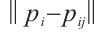 is the Euclidean distance between
  and
and  .The value sets a standard for density against which the downsampling process must compare.
2) The downsampling process can be represented by a model based on the expansion of an interval. The magnification factor m represents the ratio of the new interval to the original interval.
 (2)
(2)
Equation (2) binds m directly to the voxel size v. Consequently, deriving the optimal v is the central theoretical objective.
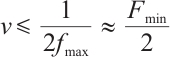
3) Through the formulation of the problem of retaining features, the Shannon-Nyquist theorem is used in connection with signal reconstruction to attain accuracy. The guiding principle states that error-free signal reconstruction must be able to capture the highest geometric frequency  , which is determined by the minimum feature size
  .
.
 (3)
(3)
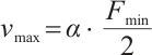
4) Considering the non-ideal nature of real-world point clouds, a robustness coefficient  is introduced to derive the maximum safe sampling interval:
 (4)
(4)
5) By substituting the voxel size formula (4) into the magnification definition (2), we obtain the final theoretical expression for the adaptive  :
:
 (5)
(5)
This formula achieves adaptive parameter setting for downsampling. The intensity of downsampling is not arbitrary; instead, it is objectively determined by the intrinsic properties of the point cloud (global point spacing  ) and the extrinsic task requirements (minimum feature size
  ).
).
Comparison of uniform voxel and Nyquist-based adaptive downsampling is shown in Fig.1.
 |
Fig. 1 Comparison of uniform voxel and Nyquist-based adaptive downsampling |
1.2 Scale-Adaptive FPFH Feature Extraction
To address the issue of low computational efficiency of traditional methods on non-uniform point clouds, this section first elucidates the calculation principle of FPFH, analyzes its bottleneck under the traditional fixed-radius strategy, and derives the acceleration mechanism of the proposed scale-adaptive method.
FPFH is an efficient operator describing the local geometric topology of point clouds. Its calculation process mainly includes the following three steps:
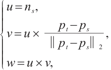
1) Local Frame Construction: For a query point  and any point
  in its neighborhood, a local coordinate system (u, v, w) is established based on the normal vector
  :
:
 (6)
(6)
where  2 denotes the L2 norm, and
  represents the cross product. The resulting
  forms the local Darboux frame for the point pair.
2) Feature Component Calculation: In the local frame, three angular features  between
  and
and  are calculated to form a Simplified Point Feature Histogram (SPFH):
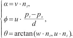 (7)
(7)
3) Neighborhood Weighted Fusion: To enhance feature descriptiveness, FPFH fuses the SPFH of the query point with those of its k-neighbors:
 (8)
(8)
where  denotes the Euclidean distance between query point
  and its neighbor point
  .
.
Figure 2 shows the FPFH feature extraction algorithm schematic diagram. Despite its effectiveness, the traditional FPFH algorithm typically sets a globally fixed search radius  . In dense regions, the number of neighbor points
  within this fixed radius grows cubically:
 (9)
(9)
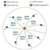 |
Fig. 2 FPFH feature extraction algorithm schematic diagram |
Since the single-point calculation time of FPFH is proportional to the number of neighbors, the total computational complexity  becomes extremely high:
 (10)
(10)
where N denotes the total number of points in the dataset, and  represents the maximum local point density.
Our method utilizes the optimal geometric description scale-voxel size v obtained from the preceding adaptive downsampling step. We dynamically bind the FPFH feature search radius r to the local voxel scale v:
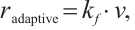 (11)
(11)
where  is a constant scaling factor used to adjust the search radius. The introduction of
  ensures that the search volume scales proportionally with the point resolution, preventing an explosion in the number of neighbor points in high-density regions and thus maintaining high computational efficiency.
This dynamic binding leads to the following properties:
1) Density Normalization: After adaptive downsampling, the local density  in any region is inversely proportional to the current voxel size v:
 (12)
(12)
2) Constant Neighbor Count: When calculating features, the number of neighbors  contained within the adaptive radius
  is derived as:
 (13)
(13)
where  denotes the volume of the adaptive search sphere, and
  represents the point density of the downsampled point cloud. The variable
  in the numerator and denominator cancels out, yielding:
 (14)
(14)
This implies that the neighbor count  degenerates into a constant C related only to the coefficient
  .
.
3) Theoretical Speedup Analysis: Since the neighbor count no longer varies with the original point cloud density  , the total time complexity
  of our method becomes
  . The theoretical speedup ratio can be expressed as:
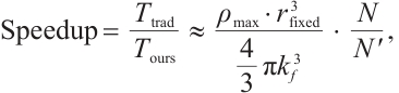 (15)
(15)
where  and
and  represent the computational time of the traditional FPFH algorithm and our method, respectively. Here,
  denotes the maximum local point density of the original point cloud, and N/N′ represents the downsampling ratio.The analysis indicates that, without sacrificing feature extraction quality, the improved algorithm achieves a clear gain in computational efficiency.
Figure 3 shows comparison of neighborhood search strategy between traditional fixed-scale FPFH and our adaptive-scale FPFH.
 |
Fig. 3 Comparison of neighborhood search strategy between traditional fixed-scale FPFH and our adaptive-scale FPFH |
1.3 ICP Registration
Fine registration is sensitive to noise and initial pose, typically relying on a high overlap ratio and local feature consistency, thus requiring a relatively accurate initial registration. After coarse registration, the ICP [16] algorithm is employed for fine registration. The procedure is as follows:
1) For each point in the source point cloud, the closest corresponding point in terms of geometric distance will be searched for within the target point cloud space.
2) Outlier correspondences with excessively large distances or those that violate geometric constraints are filtered out to enhance matching robustness.
3) Based on the remaining correspondences, the optimal rigid transformation is computed using Singular Value Decomposition (SVD).
4) The current transformation matrix is applied to align the source point cloud with the target point cloud.
5) The above process is performed iteratively until the change in pose falls below a predefined threshold or the maximum number of iterations is reached. The error function is defined as follows:
 (16)
(16)
where  represents the objective error function, R and t denote the rotation matrix and translation vector respectively, N is the total number of point correspondences, while
  and
and  are the i-th pair of corresponding points in the target and source point clouds.
2 Experiment
2.1 Experimental Environment
The dataset used in this study was acquired using a laboratory-built high-precision three-dimensional scanning system based on line-structured laser technology, as shown in Fig. 4. A Keyence LJ-30 scanning head was used for scanning the workpiece, and a resolution in the range of a micrometer was obtained. For motion control, command signals were issued by the host computer to drive the XYZ stepper motors.
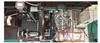 |
Fig. 4 Point cloud scanning system |
To test the registration results of the proposed algorithm, experiments were conducted on two datasets of industrial blades. The first one represents a turbopump blade with dimensions of 78.83 mm × 105.50 mm× 23.46 mm and 1 024 897 points. The other set represents a damaged compressor blade that has larger dimensions of 114.42 mm× 109.36 mm× 42.60 mm with 1 282 190 points.
The two datasets exhibit distinct feature distributions. For the turbopump blade, many points are densely distributed over non-contour regions, resulting in substantial redundancy. If conventional downsampling strategies are applied directly, this redundancy leads to unnecessary computational overhead. In contrast, the point cloud of the damaged compressor blade shows pronounced geometric features at the edges and within internal cavity regions. Under a fixed downsampling scheme, critical geometric details in these areas are prone to being lost. To address the issue, the main body of the point cloud is treated as a low-frequency signal in this study. The minimum sampling frequency is set to 0.02, which effectively removes redundant points in relatively flat regions while allocating computational resources to areas with more complex geometric features. Combined with the computed global point spacing, this strategy is applied to downsample both point cloud datasets.
Both registration experiments were conducted in an identical computational environment. The computer used was running Windows 11 with an Intel Core i5-12600KF CPU and 32 GB of RAM. All the above-mentioned algorithms were developed in Python programming using the PyCharm environment.
2.2 Qualitative Registration Results
To intuitively evaluate the registration performance, we compared the proposed method with FPFH+ICP, 3DSC+ICP, and PCA+ICP. The visualization results are presented below, where the source point cloud is rendered in red and the target point cloud is blue.
Figure 5 illustrates the registration results for the engine turbopump blades. As shown in the magnified view (top-right), the registration quality varies significantly among the algorithms. Both 3DSC+ICP and PCA+ICP exhibit visible misalignment at the curved blade tip, resulting in a distinct "ghosting" effect where the red source points and blue target points are clearly separated. This indicates that these methods failed to converge accurately on the smooth surface. In contrast, FPFH+ICP and Ours+ICP achieve a seamless alignment. The source and target point clouds are perfectly superimposed, creating a uniform overlap. This visual evidence demonstrates that our method effectively handles the high point redundancy in these smooth regions and attains high precision comparable to the classic FPFH algorithm.
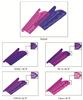 |
Fig. 5 Registration results of engine turbopump blades |
Figure 6 presents the qualitative registration results for the damaged engine compressor blades. Unlike the smooth turbopump blades, this dataset represents a more challenging scenario characterized by severe geometric discontinuities and jagged fracture edges. As observed in the magnified view (bottom-right) focusing on the fracture zone, the registration performance differs markedly among the algorithms: The 3DSC+ICP method fails to preserve the sharp geometric structure at the boundary. Due to its sensitivity to non-uniform point density, the algorithm produces a chaotic point distribution, where the source and target clouds appear scattered and unable to converge on the edge features. Similarly, the PCA+ICP algorithm exhibits clear systematic errors. A visible translational offset exists between the red source contours and the blue target contours, indicating that the global principal component analysis was insufficient to handle the local deformations caused by the damage. In sharp contrast, Ours+ICP method demonstrates superior robustness. As shown in the magnified view, our method tightly aligns with complex, irregular fracture boundaries without any "ghosting" artifacts. By dynamically adjusting the feature extraction radius, our approach effectively captures the intricate details of the damaged regions, achieving a high-precision fit that visually outperforms the comparative methods.
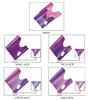 |
Fig. 6 Registration results of damaged engine compressor blades |
2.3 Quantitative Comparison and Analysis
To quantitatively evaluate the performance of the proposed algorithm, we compared it with FPFH+ICP, 3DSC+ICP, and PCA+ICP. The detailed comparison results regarding registration accuracy (Root Mean Square Error, RMSE) and computational time for both datasets are summarized in Table 1.
Accuracy Analysis: For the engine turbopump blades, the FPFH+ICP algorithm achieved the highest accuracy with an RMSE of  mm. This is expected, as the standard FPFH algorithm, with its fixed search radius, tends to capture broader contextual information in smooth regions, leading to stable feature descriptors. However, our method followed closely with an RMSE of
  mm. The marginal difference indicates that our adaptive downsampling strategy successfully retained the essential geometric information while filtering out redundant data in flat regions. Conversely, for the damaged compressor blades, the performance trend reversed. Our method outperformed FPFH+ICP, achieving the lowest RMSE of
  mm compared with that of FPFH (
 mm). This superior accuracy is attributed to the adaptive neighborhood mechanism. While FPFH employs a fixed search radius that may under-sample critical features at the sparse, jagged fracture edges, our method dynamically adjusts the search scale based on local density. This ensures that the complex geometry of the damage is accurately described, leading to a more robust registration in non-uniform regions.
Efficiency Analysis: In terms of computational efficiency, our method demonstrates a significant advantage. For the large-scale damaged blade dataset, our method required only 19.42 s, reducing the processing time by approximately 55% compared with FPFH+ICP (43.25 s). Compared with the 3DSC+ICP method, our approach requires less than 10% of the processing time. This speedup validates the theoretical analysis in Section 1: by converting the neighbor search complexity from a cubic growth function to a constant scale via density normalization, we achieve high-speed processing without sacrificing accuracy.
Comparative Performance: Regarding the other baselines, PCA+ICP was the fastest (16.62 s) but suffers from poor accuracy (magnitude of  mm), proving that global features alone are insufficient for high-precision industrial inspection. 3DSC+ICP performed the worst in both metrics, likely due to its sensitivity to point density variations, making it unsuitable for scanning data with irregular distributions.
Comparison of registration accuracy (RMSE) and computational time for different algorithms on two datasets
3 Conclusion
Aiming at the problem of low efficiency of existing algorithms in processing medium and large-scale point cloud registration, we propose an improved FPFH registration method based on dynamic downsampling and adaptive neighborhood mechanism. This method first calculates the global average point spacing based on the local density characteristics of the point cloud and then performs dynamic voxel downsampling on the original data to obtain a streamlined point cloud. Then, the neighborhood radius of the FPFH feature is dynamically adjusted according to the global average point spacing to enhance the adaptability of the feature descriptor to density changes. Based on the optimized feature set, the ICP algorithm is used to complete fine registration. Experiments show that the proposed algorithm significantly shortens the processing time while maintaining good accuracy. Contrary to fixed-radius approaches that failed at the sparse edges of the damaged compressor blade, our density-aware scheme successfully retained the critical geometric features, proving that the adaptive radius prevents information loss in non-uniform regions. Future work will extend this method to handle severe occlusion or integrate deep learning-based semantics.
References
- Liu Z, Tang H, Lin Y, et al. Point-voxel CNN for efficient 3D deep learning[J]. Advances in Neural Information Processing Systems (NeurIPS), 2019, 32: 8382-8392 . [Google Scholar]
- Chen X Y, Wu P X, Li G, et al. LIO-PPF: Fast LiDAR-inertial odometry via incremental plane pre-fitting and skeleton tracking[C]//2023 IEEE/RSJ International Conference on Intelligent Robots and Systems (IROS). New York: IEEE, 2023: 1458-1465. [Google Scholar]
- Stathopoulou E K, Battisti R, Cernea D, et al. Multiple view stereo with quadtree-guided priors[J]. ISPRS Journal of Photogrammetry and Remote Sensing, 2023, 196: 197-209. [Google Scholar]
- Liang D K, Zhou X, Xu W, et al. PointMamba: A simple state space model for point cloud analysis[J]. Advances in Neural Information Processing Systems (NeurIPS), 2024, 37:32653-32677. [Google Scholar]
- Si H Q, Qiu J X, Li Y. A review of point cloud registration algorithms for laser scanners: Applications in large-scale aircraft measurement[J]. Applied Sciences, 2022, 12(20): 10247. [Google Scholar]
- Rusu R B, Cousins S. 3D is here: Point cloud library (PCL)[C]//2011 IEEE International Conference on Robotics and Automation. New York: IEEE, 2011: 1-4. [Google Scholar]
- Wang S Z, Kannala J, Pollefeys M, et al. Guiding local feature matching with surface curvature[C]//2023 IEEE/CVF International Conference on Computer Vision (ICCV). New York: IEEE, 2024: 17935-17945. [Google Scholar]
- Hu X H, Zeng Z, Deng J W, et al. Curvature-aware point-pair signatures for robust unbalanced point cloud registration[J]. Sensors, 2025, 25(20):6267. [Google Scholar]
- Li P, Xin S, Li J, et al. A three-dimensional laser point cloud rough registration algorithm based on virtual feature points[J]. Journal of Geo-Information Science, 2018, 20(4):430-439 . [Google Scholar]
- Bellekens B, Spruyt V, Berkvens R, et al. A survey of rigid 3D point cloud registration algorithms[C]// The 4th International Conference on Ambient Computing, Applications, Services and Technologies. New York: IEEE, 2014: 8-13 . [Google Scholar]
- Huang X S, Mei G F, Zhang J, et al. A comprehensive survey on point cloud registration[EB/OL]. [2021-03-20]. https://arxiv.org/abs/2103.02690. [Google Scholar]
- Rusu R B, Blodow N, Marton Z C, et al. Aligning point cloud views using persistent feature histograms[C]//2008 IEEE/RSJ International Conference on Intelligent Robots and Systems. New York: IEEE, 2008: 3384-3391. [Google Scholar]
- Rusu R B, Blodow N, Beetz M. Fast point feature histograms (FPFH) for 3D registration[C]//2009 IEEE International Conference on Robotics and Automation. New York: IEEE, 2009: 3212-3217. [Google Scholar]
- Dong Z, Liang F, Yang B, et al. Registration of large-scaleterrestrial laser scanner point clouds: A review andbenchmark[J]. ISPRS Journal of Photogrammetry and Remote Sensing, 2020, 163: 327-342. [Google Scholar]
- Frome A, Huber D, Kolluri R, et al. Recognizing objects in range data using regional point descriptors[C]//EuropeanConference on Computer Vision (ECCV). Berlin: Springer-Verlag, 2004: 224-237. [Google Scholar]
- Besl P J, McKay N D. A method for registration of 3-D shapes[J]. IEEE Transactions on Pattern Analysis and Machine Intelligence, 1992, 14(2): 239-256. [Google Scholar]
All Tables
Comparison of registration accuracy (RMSE) and computational time for different algorithms on two datasets
All Figures
|
Fig. 1 Comparison of uniform voxel and Nyquist-based adaptive downsampling |
| In the text | |
|
Fig. 2 FPFH feature extraction algorithm schematic diagram |
| In the text | |
|
Fig. 3 Comparison of neighborhood search strategy between traditional fixed-scale FPFH and our adaptive-scale FPFH |
| In the text | |
|
Fig. 4 Point cloud scanning system |
| In the text | |
|
Fig. 5 Registration results of engine turbopump blades |
| In the text | |
|
Fig. 6 Registration results of damaged engine compressor blades |
| In the text | |
Current usage metrics show cumulative count of Article Views (full-text article views including HTML views, PDF and ePub downloads, according to the available data) and Abstracts Views on Vision4Press platform.
Data correspond to usage on the plateform after 2015. The current usage metrics is available 48-96 hours after online publication and is updated daily on week days.
Initial download of the metrics may take a while.