© Wuhan University 2026

0 Introduction

Digital images are often affected by noise during transmission, and image denoising technology is crucial to eliminating noise interference, restoring details, and enhancing visual quality. In image denoising research, a mathematical model is used to describe the noisy image process, where recovering a clean image $\mathit{X}$ from a noisy image $\mathit{Y}$ is expressed as:

$\begin{array}{c}\mathit{Y}=\mathit{X}+\widehat{\mathit{N}}\end{array}$(1)

where $\widehat{\mathit{N}}$̂ is usually assumed to be zero-mean Gaussian noise with standard deviation σ. Due to the ill-posed nature of the problem, image priors are employed to regularize the model. Via the Maximum A Posteriori (MAP) method, this regularization problem can be transformed into a minimization problem:

$\begin{array}{c}\widehat{\mathit{X}}=\underset{\mathit{X}}{\mathrm{m}\mathrm{i}\mathrm{n}}\frac{\mathrm{1}}{\mathrm{2}}\Vert \mathit{Y}-\mathit{X}{\Vert }_{\mathrm{F}}^{\mathrm{2}}+\lambda \varphi (\mathit{X})\end{array}$(2)

where the first term represents data fidelity, and the second term is called the regularization term, λ is a regularization parameter that balances the trade-off between these two terms. How to choose a good regularization functional ϕ is an active area of research in imaging science.

Previous studies have proposed various image prior models, including local smoothness, Non-Local Self-Similarity (NSS), and sparsity priors. Among these, sparse representation stands out as a representative patch-based prior. The K-SVD (Singular Value Decomposition) algorithm^[1] pioneered the application of sparse coding in image processing. The NSS prior^[2-4] exploited the structural similarity among image patches. Due to the high correlation between such patches, this prior has inspired research directions such as Low-Rank Matrix Factorization (LRMF)^[5] and Nuclear Norm Minimization (NNM)^[2,6]. Building on LRMF, methods like Rank Residual Constraint (RRC)^[7] and Group Sparse Residual Constraint (GSRC)^[8] demonstrate strong performance in image restoration tasks. Specifically, RRC models low-rank residuals and achieves favorable results across various applications,while GSRC reformulates image denoising as a problem of minimizing group sparse residuals. These LRMF-based approaches leverage the low-rank structure of image patches, which is closely related to the high correlation among patches and also supports NNM—a widely adopted low-rank approximation technique that uses the nuclear norm as a convex surrogate for matrix rank. Extending NNM, Weighted Nuclear Norm Minimization (WNNM)^[9] improves flexibility by assigning different weights to individual singular values and remains a popular method for image denoising. Furthermore, the Group Sparsity Residual Constraint with Non-Local Priors for Image Restoration (GSRC-NLP) model^[10], which is built upon GSRC, incorporates non-local priors before applying constraints on the input image, thereby achieving enhanced restoration performance.

In image denoising, the NSS prior plays a crucial role in many algorithms. These methods exploit the internal self-similar structures of an image by aggregating similar patches to extract redundant information, thereby achieving effective denoising performance. However, the NSS prior has two main limitations:

1) NSS methods typically process patch groups with identical penalty intensities, ignoring subtle differences in local structures (e.g., textures, edges, or noise levels) among patches. This "one-size-fits-all" approach fails to adapt to diverse patch characteristics, leading to suboptimal denoising results—such as artifacts or loss of fine details.

2) For highly noisy images, NSS struggles to identify sufficiently numerous or similar patches. The scarcity and low similarity of patches under high noise levels compromise denoising performance, as the prior relies on robust patch-group construction to exploit redundancy.

Our previous work on the GSRC-Log model^[11] addressed the first limitation by introducing a weighted log-sum penalty, which enables the adaptive adjustment of penalty intensities based on patch similarity. This dynamic weighting strategy preserves NSS structures in high-similarity regions while effectively suppressing noise in low-similarity regions.

To tackle the second limitation, this paper proposes a MSGSR-Log model based on multi-scale patch extraction strategy. By integrating upsampling, downsampling, and the original scale, we construct multi-scale image representations to:

1) Increase the quantity of similar patches by exploring structural similarity across resolutions.

2) Enhance patch similarity by leveraging scale-invariant features, especially in noisy scenarios where single-scale NSS struggles.

Experimental results demonstrate that the proposed MSGSR-Log model outperforms state-of-the-art methods, particularly under high noise levels, by combining adaptive weighting with multi-scale patch aggregation^[12].

1 MSGSR-Log Model for Image Denoising

1.1 Construction Process of Multi-Scale Similar Patch Groups

Firstly, we examine multi-scale image processing strategies. This strategy constructs multi-resolution image representations by performing downsampling, upsampling, and combining with the original-scale image. Specifically, downsampling reduces image resolution via pixel aggregation or mean filtering (e.g., scaling factors of 0.55 and 0.75), smoothing noise, reducing data volume, and highlighting the main structure to facilitate coarse-grained patch group matching. Upsampling employs interpolation algorithms (e.g., bilinear) to enlarge the image (e.g., scaling factors of 1.2, 1.6), improving resolution to preserve details and uncovering more potential similar structures in high-noise environments. By integrating images at different scales, this strategy captures global structural similarity through downsampling and supplements detailed similarity via upsampling, effectively mitigating the scarcity of similar patches in NSS under high-noise scenarios. It furnishes richer contextual information for image denoising and enhances denoising algorithm performance.

The multi-scale similar patch search approach complements the NSS approach by exploring similar structures at different scales. In previous multi-scale similar patch construction research, most studies employed the residual between the multi-scale similar patch group and the product of the Principal Component Analysis (PCA) dictionary matrix (based on the original image) and group sparse coefficient matrix as a regularization term in objective function minimization. Additionally, previous experiments mostly limited multi-scale processing to the coarsely downsampled scale.

Downsampling has several benefits:

1) It can smooth the image and reduce noise to a certain extent by aggregating or averaging adjacent pixels during processing.

2) Compared with upsampling, it reduces image data volume, benefiting video stream transmission, complexity reduction, and computational efficiency improvement.

3) It removes some image details, highlighting main structures and features for coarse-grained analysis.

However, downsampling also has limitations. For many images, the time required for patch extraction via upsampling and downsampling is comparable. But when multiscale similar patch group extraction is incorporated into the regularization term, upsampling increases the computational time for solving the minimization problem. In fact, when upsampling is used solely for similar patch search (not in regularization term solving), its time complexity is lower than previous downsampling based solutions. Additionally, downsampling reduces image resolution and causes aliasing effects (e.g., jagged edges). As the scaling factor decreases, textured regions in images produce more artifacts, leading to significantly worse denoising results than upsampling.

Conversely, upsampling increases resolution, clarifying details and enabling more accurate similar patch localization, thus better preserving details during denoising. Relying solely on NSS prior information often fails to yield an adequate number of similar image patches, and even if the count meets the predefined threshold, their similarity may be insufficient. To address this, multi-scale images are introduced: similar patches are extracted from scaled images and sorted by similarity, with experimental results confirming that this improvement significantly enhances denoising performance. To bridge the global noisy image $\mathit{Y}$ to the local patch groups ${\mathit{Y}}_{\mathit{i}}$ in the optimization model, the following process is implemented: Starting from the original noisy image $\mathit{Y}$, we first construct multi-scale image representations by integrating downsampled, upsampled, and the original-scale images. For each reference patch in the original image, we search across these multi-scale images using distance metrics to identify similar patches, which are then aggregated into groups. Each of these groups corresponds to a subset ${\mathit{Y}}_{\mathit{i}}$ of the global noisy image $\mathit{Y}$, where ${\mathit{Y}}_{\mathit{i}}$ denotes the noisy patches within the $i-\mathrm{t}\mathrm{h}$ group.

1.2 Application of Multi-Scale Similar Patch Groups in GSRC-Log

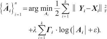
To enhance the performance of group sparse representation model, we leverage the multi-scale similar patch search strategy proposed in above subsection. For each patch group, we analyze patches across different scales by performing downsampling and upsampling, generating multi-scale image representations. At each scale, distance metrics are used to identify similar patches, expanding the set of similar patches. Building on the multi-scale similar patch groups ${\mathit{Y}}_{\mathit{i}}$ and the non-convex regularized model proposed in the GSRC-Log framework, we consider the denoising model:

$\begin{array}{c}\begin{array}{l}{\left\{{\widehat{\mathit{A}}}_{\mathit{i}}\right\}}_{i=\mathrm{1}}^n=\mathrm{a}\mathrm{r}\mathrm{g}\underset{{\mathit{A}}_{\mathit{i}}}{\mathrm{m}\mathrm{i}\mathrm{n}}\frac{\mathrm{1}}{\mathrm{2}}{\displaystyle \sum _{i=\mathrm{1}}^k}\Vert {\mathit{Y}}_{\mathit{i}}-{\mathit{X}}_{\mathit{i}}{\Vert }_{\mathrm{F}}^{\mathrm{2}}\\ +\lambda {\displaystyle \sum _{i=\mathrm{1}}^k}{\mathit{\Gamma }}_{\mathit{i}}\cdot \mathrm{l}\mathrm{o}\mathrm{g}(\left|{\mathit{A}}_{\mathit{i}}\right|+\epsilon ).\end{array}\end{array}$(3)

In Eq. (3), $k$ denotes the total number of similar-patch groups extracted from the whole image, ${\mathit{X}}_{\mathit{i}}$ represents the restored patch group from the observed noisy image ${\mathit{Y}}_{\mathit{i}},$ ${\mathit{A}}_{\mathit{i}}$ represents the group sparse coefficient of each group$X_i$, i.e., ${\mathit{X}}_{\mathit{i}}={\mathit{D}}_{\mathit{i}}{\mathit{A}}_{\mathit{i}}$. ${\mathit{D}}_{\mathit{i}}$ is an adaptive PCA dictionary learned from each patch group. The matrix ${\mathit{\Gamma }}_{\mathit{i}}$ is defined as $\mathit{I}-{\mathit{W}}_i$, where $\mathit{I}$ is an identity matrix and ${\mathit{W}}_i$ is a matrix constructed from the weights ${\mathit{\omega }}_i(j)$ that are inversely proportional to the distance between the target patch ${\mathit{y}}_{\mathit{i}}$ and its similar patch ${\mathit{y}}_i(j)$. By replicating ${\mathit{\omega }}_i(j)$ m times to form the matrix ${\mathit{W}}_i$. 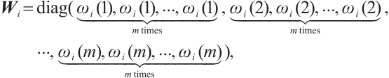This construction of ${\mathit{\Gamma }}_{\mathit{i}}$ allows the model to adaptively adjust the penalty strength based on the NSS information, which helps in preserving fine details in the image during the restoration process.The specific construction process of ${\mathit{W}}_i$ can be referred to in Eq. (4) and Eq.(5).

${\mathit{\omega }}_i(j)=\frac{\mathrm{1}}{L}\mathrm{e}\mathrm{x}\mathrm{p}\left(-\frac{\Vert y_i-y_i(j){\Vert }_{\mathrm{F}}^{\mathrm{2}}}{h^{\mathrm{2}}}\right),$(4)

$\begin{array}{l}{\mathit{W}}_i=\mathrm{d}\mathrm{i}\mathrm{a}\mathrm{g}(\underset{m\mathrm{t}\mathrm{i}\mathrm{m}\mathrm{e}\mathrm{s}}{\underbrace{{\omega }_i(\mathrm{1}),{\omega }_i(\mathrm{1}),...,{\omega }_i(\mathrm{1})}},\underset{m\mathrm{t}\mathrm{i}\mathrm{m}\mathrm{e}\mathrm{s}}{\underbrace{{\omega }_i(\mathrm{2}),{\omega }_i(\mathrm{2}),...,{\omega }_i(\mathrm{2})}},\\ ...,\underset{m\mathrm{t}\mathrm{i}\mathrm{m}\mathrm{e}\mathrm{s}}{\underbrace{{\omega }_i(m),{\omega }_i(m),...,{\omega }_i(m)}}),\end{array}$(5)

where $L={\displaystyle \sum _{j=\mathrm{1}}^m}\mathrm{e}\mathrm{x}\mathrm{p}\left(-\frac{\Vert y_i-y_i(j){\Vert }_{\mathrm{F}}^{\mathrm{2}}}{h^{\mathrm{2}}}\right)$ is the normalization factor, $h$ is a predefined smoothing parameter, $m$ is the number of patches per group, $y_i$ is the reference patch, and $y_i(j)$ is the $j-\mathrm{t}\mathrm{h}$ similar patch.

Due to the orthogonality of the PCA dictionary ${\mathit{D}}_i$ and the unitary invariant property of F-norm, Eq. (3) is equivalent to

$\begin{array}{c}{\widehat{\mathit{\alpha }}}_i(j)=\underset{{\mathit{\alpha }}_{\mathit{i}}(\mathit{j})}{\mathrm{a}\mathrm{r}\mathrm{g}\mathrm{m}\mathrm{i}\mathrm{n}}\frac{\mathrm{1}}{\mathrm{2}\lambda }|{\mathit{s}}_i(j)-{\mathit{\alpha }}_i(j){|}^{\mathrm{2}}+{\mathit{\gamma }}_i(j)\mathrm{l}\mathrm{o}\mathrm{g}(|{\mathit{\alpha }}_i(j)|+\epsilon )\end{array}$(6)

Notably, ${\mathit{\gamma }}_i\mathrm{l}\mathrm{o}\mathrm{g}$ is a parameterized regularization that can adjust the penalty intensity according to block similarity and control the convexity of the objective function. ε is a very small positive number used to prevent division by zero. ${\mathit{s}}_i(j)$ refers to the $j-\mathrm{t}\mathrm{h}$ element of the vectorized form of the observed noisy patch group ${\mathit{Y}}_i$, ${\mathit{\alpha }}_i(j)$ represents the sparse coefficients associated with the $j-\mathrm{t}\mathrm{h}$ element of the $i-\mathrm{t}\mathrm{h}$ patch group in the image. In image denoising experiments, it improves metrics such as Peak Signal to Noise Ratio (PSNR) and visual effects, effectively addressing the drawbacks of the unified weight in NSS.

${\mathit{A}}_i$ achieves a closed-form solution by minimizing the objective function. Drawing on the derivation of the GSRC-Log model^[11], the formula is expressed as:

${\mathit{A}}_i=\mathrm{a}\mathrm{r}\mathrm{g}\underset{A_i}{\mathrm{m}\mathrm{i}\mathrm{n}}\frac{\mathrm{1}}{\mathrm{2}}\Vert {\mathit{Y}}_i-{\mathit{D}}_i{\mathit{A}}_i{\Vert }_{\mathrm{F}}^{\mathrm{2}}+\lambda \cdot {\mathit{\Gamma }}_i\odot \mathrm{l}\mathrm{o}\mathrm{g}(\left|{\mathit{A}}_i\right|+\epsilon ).$(7)

The element-wise closed-form solution (where ${\alpha }_i(j)$denotes the $j-\mathrm{t}\mathrm{h}$ element of ${\mathit{A}}_{\mathit{i}})$ is expressed as:$\begin{array}{l}{\alpha }_i(j)=\mathrm{P}\mathrm{r}\mathrm{o}{\mathrm{x}}_{\lambda {\gamma }_i(j)\mathrm{l}\mathrm{o}\mathrm{g}(\cdot )}(s_i(j))=\mathrm{s}\mathrm{i}\mathrm{g}\mathrm{n}(s_i(j))\cdot a\\ \cdot \mathrm{s}\mathrm{i}\mathrm{g}\mathrm{n}\left(\mathrm{m}\mathrm{a}\mathrm{x}\left\{F(a),\mathrm{0}\right\}\right)\cdot \mathrm{s}\mathrm{i}\mathrm{g}\mathrm{n}\left(\mathrm{m}\mathrm{a}\mathrm{x}\left\{{\zeta }_i(j)-\mathrm{4}{v}_i(j),\mathrm{0}\right\}\right),(\mathrm{8})\end{array}$

where:

$a=\frac{{\zeta }_i(j)+\sqrt[]{{\zeta }_i(j)-\mathrm{4}{v}_i(j)}}{\mathrm{2}},$(9)

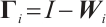${\zeta }_i(j)=s_i(j)-\epsilon$, where $s_i(j)$ is the $j-\mathrm{t}\mathrm{h}$ element of the vectorized ${\mathit{Y}}_i$; $v_i(j)=\lambda {\gamma }_i(j)-\epsilon s_i(j)$, and ${\gamma }_i(j)$is the $j-\mathrm{t}\mathrm{h}$ element of the vectorized ${\mathbf{\Gamma }}_i=I-{\mathit{W}}_i$; $F({\alpha }_i(j))=J(\mathrm{0})-J({\alpha }_i(j))$ , which is used to determine the global optimum. $J(\cdot )$ denotes the objective function of Eq. (6); $\mathrm{P}\mathrm{r}\mathrm{o}{\mathrm{x}}_{\cdot }$ is the proximal operator, facilitating efficient solution of optimization problems with non-convex logarithmic penalty terms; $\mathrm{s}\mathrm{i}\mathrm{g}\mathrm{n}(\cdot )$ is the sign function, ensuring consistency between the solution and the sign of $s_i(j)$.

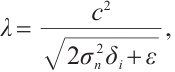
The regularization parameter $\lambda$ dynamically balances the data fidelity term and the regularization term, which is adaptively adjusted by the estimated standard deviation ${\delta }_i$ of the patch group coefficients and the noise variance ${\sigma }_n^{\mathrm{2}}$. The formula is:

$\lambda =\frac{c^{\mathrm{2}}}{\sqrt[]{\mathrm{2}{\sigma }_n^{\mathrm{2}}{\delta }_i+\epsilon }},$(10)

where $c$ is the step-size ratio parameter (adjusted according to noise levels, refer to Table 1 for values), ${\sigma }_n^{\mathrm{2}}$ is the variance of additive noise in the image, ${\delta }_i$ denotes the estimated standard variance of ${\mathit{A}}_i$, and $\epsilon$ is a tiny positive number to avoid denominator zero.

The GSRC-Log method employs a group-sparse residual constraint model with a weighted log-sum penalty, which adjusts the penalty intensity by leveraging NSS information: the denoising intensity is reduced in regions with high NSS coefficients to preserve inherent NSS structures and fine details, while being increased in regions with low NSS coefficients to enhance noise suppression. The $\mathit{\gamma }$ log regularization term^[11] is vital for this adaptive adjustment. When $\mathit{\gamma }$ is small, the local patches closely resemble the reference patches, reducing the penalty for sparse coefficients and maintaining details related to high NSS coefficients. As $\mathit{\gamma }$ increases, the convexity of the objective function changes, imposing a higher penalty on low NSS coefficients and suppressing noise. Figure 1 depicts the complete workflow of our image denoising method. Initially, we utilize the example image and its zoomed version. By employing block matching, we identify similar patches in both the original image and the zoomed image. These similar patches are subsequently subjected to multiscale similar block bonding. Following this step, we perform the SVD and utilize a PCA dictionary. Subsequently, we derive the group sparse code ${\mathit{A}}_{\mathit{i}}$ and apply the GSRC-Log for denoising, as shown in Eq. (3). After denoising, we obtain clean similar patches, from which we select blocks of the original size. Finally, we aggregate these blocks to reconstruct the clean image.

Fig. 1 Flowchart of the proposed MSGSR-Log for image denoising

To conclude this section, we provide a concise overview of Algorithm 1, namely the MSGSR-Log algorithm designed for image denoising. The MSGSR-Log algorithm significantly enhances the denoising performance by incorporating a multi-scale strategy. Specifically, it constructs multi-scale image representations by performing both downsampling and upsampling operations. Subsequently, it identifies similar patches across different scales and aggregates them into groups. A weighted logarithmic sum penalty is then applied to adaptively adjust the penalty intensity according to the similarity of the patches. This adaptive weighting mechanism enables the algorithm to preserve structural details in high-similarity regions while effectively suppressing noise in low-similarity regions. By leveraging the strengths of both the GSRC-Log model and multi-scale patch aggregation, the MSGSR-Log algorithm achieves superior denoising results, particularly under high noise levels. Note that other parameter names in Algorithm 1 are consistent with those in GSRC-Log^[11].

Algorithm 1 The MSGSR-Log algorithm for image denoising

Require: The noisy image $\mathit{Y}$ 1.Initialize ${\widehat{\mathit{x}}}^{(0)}=\mathit{Y}$ and parameters $m$, $c$, h, $\lambda$ , $\epsilon$ , ρ , α and Iter. 2.for $t=0$ to Iter do 3.Divide ${\mathit{x}}^{(\mathit{t})}$ into patches $\{{\mathit{x}}_i{\}}_{i=1}^m$. 4.for each ${\mathit{x}}_i$ do 5.Construct multi-scale group ${\mathit{Y}}_{\mathit{i}}$ by integrating downsampled, upsampled, and original-scale images: 6.Step 1: Extract the original-scale patch ${{\mathit{x}}_i}^{(\mathrm{o}\mathrm{r}\mathrm{i}\mathrm{g})}$ from ${\mathit{x}}^{(t)}$ centered at the current pixel. 7.Step 2: Downsample ${\mathit{x}}^{(t)}$ using a scaling factor α (e.g., 0.55, 0.75) to obtain a lower resolution image ${\mathit{x}}^{(\mathrm{d}\mathrm{o}\mathrm{w}\mathrm{n})}$. 8.Step 3: Extract the downsampled patch ${{\mathit{x}}_{\mathit{i}}}^{(\mathrm{d}\mathrm{o}\mathrm{w}\mathrm{n})}$ from ${\mathit{x}}^{(\mathrm{d}\mathrm{o}\mathrm{w}\mathrm{n})}$ centered at the corresponding pixel. 9.Step 4: Upsample ${\mathit{x}}^{(t)}$ using a scaling factor α (e.g., 1.2, 1.6) to obtain a higher resolution image ${\mathit{x}}^{(\mathrm{u}\mathrm{p})}$. 10.Step 5: Extract the upsampled patch ${{\mathit{x}}_i}^{(\mathrm{u}\mathrm{p})}$ from ${\mathit{x}}^{(\mathrm{u}\mathrm{p})}$ centered at the corresponding pixel. 11.Step 6: Combine ${{\mathit{x}}_i}^{(\mathrm{o}\mathrm{r}\mathrm{i}\mathrm{g})}$, ${{\mathit{x}}_i}^{(\mathrm{d}\mathrm{o}\mathrm{w}\mathrm{n})}$, and ${{\mathit{x}}_i}^{(\mathrm{u}\mathrm{p})}$ to form the multi-scale group ${\mathit{Y}}_i$. 12.end for 13.for each group ${\mathit{Y}}_i$ do 14.Compute similarity weights${\mathit{\omega }}_i(j)$ by Eq. (4). 15.Construct weight matrix ${\mathit{W}}_i$ by Eq. (5). 16.Update ${\mathit{\Gamma }}_i$ by ${\mathit{\Gamma }}_i=I-{\mathit{W}}_i$. 17.Update regularization parameters [λ] by Eq. (10). 18.Construct dictionary ${\mathit{D}}_i$ by ${\mathit{Y}}_i$ using PCA. 19.Estimate ${\mathit{A}}_{\mathit{i}}$ by Eq. (8). 20.Reconstruct clean patch group: ${\widehat{\mathit{X}}}_i={\mathit{D}}_i{\widehat{\mathit{A}}}_i$​. 21.end for 22.Aggregate all ${\widehat{\mathit{X}}}_i$: Place patches back to original positions and average overlapping pixels to get ${\mathit{X}}^{(t)}$. 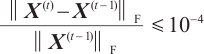23.if $\frac{\Vert {\mathit{X}}^{(t)}-{\mathit{X}}^{(t-1)}{\Vert }_{\mathrm{F}}}{\Vert {\mathit{X}}^{(t-1)}{\Vert }_{\mathrm{F}}}\le {10}^{-4}$ or $t>\mathrm{I}\mathrm{t}\mathrm{e}\mathrm{r}$ 24.break 25.end if 26.end for 27.Output: Restored image $\widehat{\mathit{x}}$.

2 Experiment

In this section, we present the experimental results of introducing multi-scale similar block matching based on GSRC-Log. The specific experiments are divided into two parts.

First, we degraded the test images by adding zero-mean white Gaussian noise to generate noisy observation images. We reported the results of denoising at different noise levels ($\sigma$ = 30, 50 and 75) and compared them with state of the art denoising methods, including BM3D^[13], NCSR^[14], SAIST^[15], EPLL^[16], PGPD^[17], RRC^[7], GSRC-NLP^[9], and GSRC-Log^[11]. To evaluate the quality of the restored images, we used both the Peak Signal to Noise Ratio (PSNR) and the Structural Similarity Index (SSIM) as references. For the selection of database images, we followed the same approach as GSRC-Log. Table 1 lists the algorithmic parameters adopted for different noise levels. τ is the ADMM penalty coefficient, ρ controls the curvature of the logarithmic regularizer, c gives the step-size ratio of the searching window, m and h are the maximum number of patches per group and the half-size of the search window, respectively, and $\sqrt[]{b}$ is the square-root of the PCA dictionary atom count. Their values are adaptively tuned according to the noise standard deviation σ.

Secondly, to verify the better denoising performance of introducing multi-scale similar block matching under large noise variances, since GSRC-Log has already demonstrated excellent denoising and texture preserving capabilities. Meanwhile, we conduct a comparison of PSNR and SSIM under the condition of relatively high noise levels ($\sigma$ =100). In addition, we calculate the differences between these two metrics for the two denoising methods. To control the experimental variables, the search window used in the block matching process was kept the same as that of GSRC-Log, with a size of 25×25. Other parameter settings were also consistent with those of GSRC-Log. That is, we only changed the scale size and the ratio between the original scale and the scaled scale. In terms of multi-scale scaling ratios, we selected eight scaling factors: 0.55, 0.65, 0.75, 0.90, 1.05, 1.20, 1.40, and 1.60. The specific parameter settings are provided in Table 2.

The denoising method we proposed has been comprehensively compared with a series of traditional and state-of-the-art denoising methods, such as BM3D, EPLL, NCSR and PGPD, at different noise levels. The experimental results are shown in Table 3 and Table 4.

From the results in Table 3, it can be seen that for various test images, the method proposed in this paper achieves superior PSNR and SSIM values across different noise levels compared with other methods. On average, it outperforms other comparative methods by a certain margin, which fully demonstrates the outstanding ability of our method to restore the true image signals and minimizes the distortion effects caused by noise to the greatest extent. Regarding SSIM, an important dimension for evaluating the structural similarity of images, our method also performs remarkably well. Whether we are dealing with texture-rich images with abundant details or images containing complex scenes, under various noise conditions, the SSIM values of the images processed by our method are closer to 1. This indicates that the generated denoised images are more similar to the original images in terms of both structure and visual perception, and our method can better preserve the details and structural information of the images.

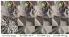Fig. 2 Denoising results at $\mathit{\sigma }$ = 100 (Barbara) (a) Noise image; (b) PSNR=23.05 dB and SSIM=0.612 4; (c) PSNR=23.35 dB and SSIM=0.626 8; (d) PSNR=23.62 dB and SSIM=0.642 1.

Fig. 3 Denoising results at $\mathit{\sigma }$ = 100 (Brodatz) (a) Noise image; (b) PSNR=19.07 dB and SSIM=0.518 8; (c) PSNR=19.22 dB and SSIM=0.530 5; (d) PSNR=19.42 dB and SSIM=0.562 9.

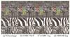Fig. 4 Denoising results at $\mathit{\sigma }$ = 100 (Zebra) (a) Noise image; (b) PSNR=19.51 dB and SSIM=0.537 6; (c) PSNR=19.63 dB and SSIM=0.553 1; (d) PSNR=19.81 dB and SSIM=0.569 3.

It is particularly worth noting that, as evidenced by the experimental results in Table 5, the D-value represents the difference between our method and GSRC-Log in both PSNR and SSIM measures, our method demonstrates extremely strong superiority under conditions of high noise levels. This validates our previous conjecture. When confronted with high noise levels, the NNS prior fails to identify a sufficient number of similar patches, and the degree of similarity among these patches does not meet the expected standards. In contrast, our method can perfectly address the limitations of the NSS in such scenarios. Figures 2-5 illustrate the denoising details in a noise state of $\sigma$ = 100. It can be intuitively perceived that our algorithm has more powerful advantages in terms of texture clarity and background details. For texture-rich images like Barbara and Brodatz, the multi-scale strategy of MSGSR-Log amplifies subtle texture structures, making it easier to identify similar patches even under high noise.

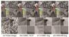Fig. 5 Denoising results at σ = 100 (Flower) (a) Noise image; (b) PSNR=22.36 dB and SSIM=0.584 4; (c) PSNR=22.60 dB and SSIM=0.594 8; (d) PSNR=22.77 dB and SSIM=0.605 3.

By integrating the experimental results from these two key dimensions, PSNR and SSIM, the denoising method we proposed exhibits significant advantages. Not only does it demonstrate excellent noise removal performance, but it also surpasses many existing traditional and advanced denoising methods to maintain and enhance image quality. This provides a more promising solution for the development of image denoising technology. For smooth images such as Windows, the original NSS already captures sufficient similar patches in the single scale. Multi-scale sampling adds limited effective information.

Although the multi-scale strategy improves performance, it inevitably increases the computing burden. Table 6 therefore reports the actual CPU time measured on the same workstation (CPU: i9-13980HX and GPU:4060 laptop). For the four noise levels ($\sigma$ = 30, 50, 75, 100) the proposed MSGSR-Log needs on average 220.58 s, which is 2.85 times that of the single-scale GSRC-Log (77.42 s). In practice the extra cost is acceptable on a standard PC when a parfor (parallel for loop, a parallel computing construct) version (Utilize 12 cores) is used (approximately 1.44 times). Consequently, it is recommended for applications where quality is the primary concern.

3 Sensitivity Analysis——Zoom Scale

To further evaluate the sensitivity of the proposed MSGSR-Log model to different scaling factors, we conducted experiments to analyze how varying scaling factors (denoted by k) affect image denoising performance in Table 7. Specifically, we selected ten scaling factors (k= 0.55, 0.65, 0.75, 0.90, 1.05, 1.20, 1.40, and 1.60) and applied the MSGSR-Log model to a subset of images under a noise level of $\sigma$ = 75. The resulting PSNR and SSIM values were recorded for comparison. The optimal values for each item have been highlighted in bold.

The experimental results indicate that the MSGSR-Log model maintains relatively stable performance across different scaling factors, but optimal performance is image-dependent. For texture-rich images such as Brodatz , larger upsampling factors (e.g., 1.4 or 1.6) tend to preserve more structural details, leading to higher PSNR and SSIM values. In contrast, for images with simpler structures, moderate scaling factors (e.g., 0.9 or 1.2) yield more consistent and reliable results.

Moreover, we observe that extreme scaling factors—either too large (>1.6) or too small (<0.55)—can lead to performance degradation. This is likely due to structural distortion or inaccurate patch matching, which undermines the effectiveness of sparse representation and residual constraint modeling.

In summary, while the MSGSR-Log model demonstrates robustness to scale variation, selecting an appropriate scaling factor based on image content characteristics can further enhance denoising performance. Table 7 presents the PSNR and SSIM values of selected images under different scaling factors, offering a clear visualization of this sensitivity trend. The source code of our MSGSR-Log for image denoising is available at https://github.com/zt9877.

4 Conclusion

This paper presents the MSGSR-Log model, a novel approach for image denoising that integrates multi-scale patch analysis with a weighted log-sum penalty. The model effectively leverages the NSS prior to enhance denoising performance, particularly under high noise conditions. By dynamically adjusting penalties based on patch similarity, MSGSR-Log preserves texture details and suppresses noise, outperforming state-of-the-art methods. The experimental results validate the model's superiority in terms of PSNR and SSIM, demonstrating its robustness and effectiveness in various noisy scenarios. Moreover, the multi-scale patch analysis and adaptive penalty mechanism address the limitations of traditional NSS-based methods, which often fail to identify sufficient similar patches and maintain high similarity under high noise levels.

References

All Tables

All Figures

	Fig. 1 Flowchart of the proposed MSGSR-Log for image denoising
In the text

	Fig. 2 Denoising results at $\mathit{\sigma }$ = 100 (Barbara) (a) Noise image; (b) PSNR=23.05 dB and SSIM=0.612 4; (c) PSNR=23.35 dB and SSIM=0.626 8; (d) PSNR=23.62 dB and SSIM=0.642 1.
In the text

	Fig. 3 Denoising results at $\mathit{\sigma }$ = 100 (Brodatz) (a) Noise image; (b) PSNR=19.07 dB and SSIM=0.518 8; (c) PSNR=19.22 dB and SSIM=0.530 5; (d) PSNR=19.42 dB and SSIM=0.562 9.
In the text

	Fig. 4 Denoising results at $\mathit{\sigma }$ = 100 (Zebra) (a) Noise image; (b) PSNR=19.51 dB and SSIM=0.537 6; (c) PSNR=19.63 dB and SSIM=0.553 1; (d) PSNR=19.81 dB and SSIM=0.569 3.
In the text

	Fig. 5 Denoising results at σ = 100 (Flower) (a) Noise image; (b) PSNR=22.36 dB and SSIM=0.584 4; (c) PSNR=22.60 dB and SSIM=0.594 8; (d) PSNR=22.77 dB and SSIM=0.605 3.
In the text

References

- Elad M, Aharon M. Image denoising via sparse and redundant representations over learned dictionaries[J]. IEEE Transactions on Image Processing, 2006, 15(12): 3736-3745. [NASA ADS] [CrossRef] [MathSciNet] [PubMed] [Google Scholar]
- Mairal J, Bach F, Ponce J. Non-local sparse models for image restoration[C]//Proc IEEE 12th Int Conf Comput Vis. New York: IEEE, 2009: 2272-2279. [Google Scholar]
- Buades A, Coll B, Morel J M. A non-local algorithm for image denoising[C]//2005 IEEE Computer Society Conference on Computer Vision and Pattern Recognition (CVPR'05). New York: IEEE, 2005: 60-65. [Google Scholar]
- Zhang J, Zhao D, Gao W, et al. Group-based sparse representation for image restoration[J]. IEEE Trans Image Process, 2014, 23(8): 3336-3351. [Google Scholar]
- Srebro N, Jaakkola T. Weighted low-rank approximations[C]// Proceedings of the Twentieth International Conference on International Conference on Machine Learning, ICML'03. Cambridge: AAAI Press, 2003: 720-727. [Google Scholar]
- Hu Y, Zhang D B, Ye J P, et al. Fast and accurate matrix completion via truncated nuclear norm regularization[J]. IEEE Transactions on Pattern Analysis and Machine Intelligence, 2013, 35(9): 2117-2130. [Google Scholar]
- Zha Z Y, Yuan X, Wen B H, et al. From rank estimation to rank approximation: Rank residual constraint for image restoration[J]. IEEE Transactions on Image Processing, 2020, 29: 3254-3269. [Google Scholar]
- Zha Z Y, Liu X, Zhou Z H, et al. Image denoising via group sparsity residual constraint[C]//2017 IEEE International Conference on Acoustics, Speech and Signal Processing (ICASSP). New York: IEEE, 2017: 1787-1791. [Google Scholar]
- Gu S H, Zhang L, Zuo W M, et al. Weighted nuclear norm minimization with application to image denoising[C]//2014 IEEE Conference on Computer Vision and Pattern Recognition. New York: IEEE, 2014: 2862-2869. [Google Scholar]
- Zha Z Y, Yuan X, Wen B H, et al. Group sparsity residual constraint with non-local priors for image restoration[J]. IEEE Transactions on Image Processing, 2020, 29: 8960-8975. [NASA ADS] [CrossRef] [MathSciNet] [Google Scholar]
- Zhang T, Li W Y, Wu D, et al. Group sparsity residual constraint model with weighted log-sum penalty for image restoration[J]. Signal Processing, 2024, 222: 109536. [Google Scholar]
- Ning W, Sun D, Gao Q W, et al. Natural image restoration based on multi-scale group sparsity residual constraints[J]. Frontiers in Neuroscience, 2023, 17: 1293161. [Google Scholar]
- Dabov K, Foi A, Katkovnik V, et al. Image denoising by sparse 3-D transform-domain collaborative filtering[J]. IEEE Transactions on Image Processing, 2007, 16(8): 2080-2095. [CrossRef] [Google Scholar]
- Dong W S, Zhang L, Shi G M, et al. Nonlocally centralized sparse representation for image restoration[J]. IEEE Transactions on Image Processing, 2013, 22(4): 1620-1630. [Google Scholar]
- Dong W S, Shi G M, Li X. Nonlocal image restoration with bilateral variance estimation: A low-rank approach[J]. IEEE Transactions on Image Processing, 2013, 22(2): 700-711. [NASA ADS] [CrossRef] [MathSciNet] [PubMed] [Google Scholar]
- Zoran D, Weiss Y. From learning models of natural image patches to whole image restoration[C]//2011 International Conference on Computer Vision. New York: IEEE, 2012: 479-486. [Google Scholar]
- Xu J, Zhang L, Zuo W M, et al. Patch group based nonlocal self-similarity prior learning for image denoising[C]//2015 IEEE International Conference on Computer Vision (ICCV). New York: IEEE, 2016: 244-252. [Google Scholar]
All Tables
PSNR (dB) and SSIM comparison between GSRC-Log and MSGSR-Log for image denosing with high intensity noise ( =100)
Performance comparison of the MSGSRC-Log algorithm and the GSRC-Log algorithm under different scale factors with =75