| Issue |
Wuhan Univ. J. Nat. Sci.
Volume 27, Number 6, December 2022
|
|
|---|---|---|
| Page(s) | 453 - 464 | |
| DOI | https://doi.org/10.1051/wujns/2022276453 | |
| Published online | 10 January 2023 | |
CLC number: TP 183
A Fault Diagnosis Model for Complex Industrial Process Based on Improved TCN and 1D CNN
1
School of Electronic and Electrical Engineering, Shanghai University of Engineering Science, Shanghai 201600, China
2
State Grid Shanghai Municipal Electric Power Company, Shanghai 200122 , China
3
CSG Smart Science & Technology Co., LTD., Shanghai 201203, China
† To whom correspondence should be addressed. E-mail: This email address is being protected from spambots. You need JavaScript enabled to view it.
Received:
10
September
2022
Abstract
Fast and accurate fault diagnosis of strongly coupled, time-varying, multivariable complex industrial processes remain a challenging problem. We propose an industrial fault diagnosis model. This model is established on the base of the temporal convolutional network (TCN) and the one-dimensional convolutional neural network (1DCNN). We add a batch normalization layer before the TCN layer, and the activation function of TCN is replaced from the initial ReLU function to the LeakyReLU function. To extract local correlations of features, a 1D convolution layer is added after the TCN layer, followed by the multi-head self-attention mechanism before the fully connected layer to enhance the model's diagnostic ability. The extended Tennessee Eastman Process (TEP) dataset is used as the index to evaluate the performance of our model. The experiment results show the high fault recognition accuracy and better generalization performance of our model, which proves its effectiveness. Additionally, the model's application on the diesel engine failure dataset of our partner's project validates the effectiveness of it in industrial scenarios.
Key words: fault diagnosis / temporal convolutional network / self-attention mechanism / convolutional neural network
Biography: WANG Mingsheng, male, Master candidate, research direction: fault diagnosis. E-mail: This email address is being protected from spambots. You need JavaScript enabled to view it.
Supported by the Scientific and Technological Innovation 2030 — Major Project of "New Generation Artificial Intelligence" (2020AAA0 109300)
© Wuhan University 2022
 This is an Open Access article distributed under the terms of the Creative Commons Attribution License (https://creativecommons.org/licenses/by/4.0), which permits unrestricted use, distribution, and reproduction in any medium, provided the original work is properly cited.
0 Introduction
With the development of Industry 4.0 and intelligent manufacturing, industrial equipment has become increasingly integrated, complex, and intelligent; along with the rapid growth in the quantity of data, the performance of equipment failure is becoming more complex. The failure of complex precision industrial equipment often causes immense losses, so the accurate diagnosis of its failure is increasingly becoming a research priority.
Commonly used fault diagnosis methods are mainly divided into model-based, knowledge-based, and data-driven methods[1]. Model-based methods establish mathematical models for equipment, such as state space equations[2,3], to study different dynamic parameters and responses of equipment in normal and faulty states; knowledge-based reasoning methods are used in the case of having obtained prior knowledge of equipment failures; by combining practical experience, system principles and historical fault information, these methods can infer the reason of failure, such as fault trees based on Bayesian networks[4,5]; data-driven methods extract features from the collected historical fault data of equipment to diagnose faults, such as K-means clustering algorithm[6,7], principal component analysis (PCA) algorithm[8,9] and so on. The model-based method requires professional knowledge of the relevant equipment to establish models, yet the model is complex, with poor adaptability and reliability, and is prone to false positives and false negatives; the fault diagnosis method based on knowledge reasoning relies heavily on the prior knowledge of equipment faults, which requires a combination of a lot of practical experience to identify faults, and are often unidentifiable for unknown faults. With the continuous breakthrough of deep learning technology in image and natural language processing[10-15], the application of deep learning technology to fault diagnosis to improve its efficiency and accuracy has become a research hotspot currently. In the past literature, the recurrent neural networks (RNN)[16] like Long-Short Term Memory (LSTM)[17] network and Gate Recurrent Unit (GRU)[18] network are the commonly used deep learning networks in fault diagnosis. However, the deep RNN models face the problems of gradient disappearance and gradient explosion[19-21], and due to the dependence on the previous time step, RNN models have worse parallelization capability.
As CNN models have caught attention in time series processing recently, Wu et al[22] firstly introduced a deep convolutional neural network (CNN) to multivariate time series fault diagnosis, which formed the data into [variate, time step] matrix to apply two-dimensional convolution, and achieved 88.2% accuracy on test set; Song et al[23] used a multi-scale two-dimensional convolution to identify chemical process faults and achieved 88.54% accuracy on test set; Deng et al[24] introduced a genetic algorithm to reorder features before CNN and achieved 89.72% accuracy on the test set. These CNN models use two-dimensional convolution and pooling layers to identify faults, which may face accuracy loss and still have room for improvement. The temporal convolutional network (TCN) proposed by Bai et al[25] uses dilated convolution to better perceive long sequences and exceed LSTM and GRU in time-series prediction tasks. However, TCN can only process one-dimensional time-series data and cannot process multi-dimensional complex industrial data.
In order to accurately identify the faults in a complex multivariate industrial process that are strongly coupled and time-varying, a fault identification model based on improved TCN and one-dimensional convolution is proposed. In the model, the activation function of TCN is replaced by the LeakyReLU function, an extra one-dimensional convolution layer is introduced in the feature dimension to extract local correlation features, and the multi-head self-attention layer is introduced before the fully connected layer to establish a TCN-1DCNN-Attention (TCA) model. Finally, the effectiveness and generalization of this model are checked on by comparing the fault recognition rate with traditional RNN models like LSTM, GRU and Transformer model.
The paper is organized in the following order: Section 1 is the introduction of preliminaries, including TCN and Attention. Section 2 is the comprehensive description of our proposed model. Section 3 is the experiments and analysis, and Section 4 is the conclusion.
1 Preliminary
1.1 Temporal Convolutional Neural Network
TCN is improved on the base of the Time-Delay Neural Network (TDNN) proposed by Waibel et al[26], which has been widely used in time series modeling[27-29]. TDNN is composed of one-dimensional fully convolutional layers and causal convolution, but if we want to achieve an effective perception of long sequence data, an extremely deep network or a large convolution kernel is a necessity. To solve this problem, TCN adds dilated convolutions to achieve an exponential receptive field by inserting 0 taps between the taps of the convolution kernel.
Figure 1 shows the principle of dilated casual convolution of TCN. By using 3-layer one-dimensional casual convolution with dilation factors d=1,2,4 and filter size k=3, every tap of the output layer achieves a receptive field of 15 input data.
 |
Fig. 1 Dilated convolution |
Specifically, for a given input 1D time-series data  and convolution kernel
  , a single dilated convolution operation on sequence element s is:
 (1)
(1)
where d is the dilation factor, k is the convolution kernel size, f(i) is the i-th tap of the convolution kernel, and  is the data in the sequence corresponding to the casual convolution kernel tap, whose sample interval between taps is d.
Therefore, the dilated convolution is to add a fixed step interval to the adjacent convolution kernel taps. Specially, on the condition of dilation factor  , the dilated convolution is equivalent to a normal full convolution. In addition, to ensure the effective transfer of temporal information, TCN introduces additional residual connections. The causal convolution ensures that the convolution is carried out from the past to the future, and future data will not be introduced into the historical data; the residual connection conducts 1*1 convolution for the input data and adds the dilated convolution data to the output to realize cross-layer information transfer[30]. As a result, more historical details are obtained to improve model accuracy. Figure 2 below shows us the residual connection structure of TCN.
 |
Fig. 2 The residual connection of TCN |
Advantages of TCN are as follows:
Strong parallelism: Convolutional neural networks adopt the same convolution kernel in each layer, and long input sequences can be processed in parallel as a whole.
Flexible receptive field: The receptive field can be flexibly changed by stacking dilated convolution layers, increasing the dilation coefficient, and enlarging the convolution kernel.
Gradient stability: Different layers have different parameters and gradients and will not cause gradients to explode or disappear due to parameter sharing like RNN.
Low memory requirement: No memory unit is required except the convolution kernels, and convolution kernels are shared among the same layers, contributing to low memory requirement.
Variable input length: Input data is received by sliding one-dimensional convolution, and zero data can be automatically padded when the input sequence length is insufficient, so any data at any length can be received.
In the industrial process, a random occurrence of fault means a unfixed fault sequence length, and TCN can process these time series fault data of different lengths flexibly. Due to the parallelism and lower memory requirements, the TCN model's training requires fewer resources, which means less training time. In addition, the residual connection of TCN can better convey historical information of long-term series data to learn more features.
1.2 Multi-Head Self-Attention Mechanism
As input features increase, to obtain global feature correlation, the traditional convolutional neural network requires a very deep network, which will significantly increase model size, while the self-attention mechanism can directly obtain the global feature correlation and assign a higher weight to important information. Self-attention mechanisms require fewer parameters than other neural networks.
The essence of the self-attention mechanism is to map the input matrix  into a query matrix
  , a key matrix
  , and a value matrix
  through the matrix
  ,
,  ,
,  [31]. By multiplying the mapped matrix
  with
with  and the following softmax normalization ,we obtain the corresponding weight coefficient
  for
for  , and then
  can be weighted and summed to the attention result, as shown in formula (2):
 (2)
(2)
where  is used to prevent the gradient from disappearing, for the result of matrix multiplication is too large. In practice, single-head self-attention often pays too much attention to itself and omits detailed information, so the multi-head self-attention mechanism[13] is proposed to solve this issue. Compared with the single-head one, the multi-head self-attention can extract information at different levels, effectively improving model diagnostic performance.
Multi-head self-attention uses multiple sets of self-attention to process the input sequence, then concatenates the results and performs a linear transformation to output. Take  head self-attention as an example, its calculation process is shown in formula
  :
:
 (3)
(3)
where  is the result of i-th head self-attention, and
  is the linear transformation matrix.
 (4)
(4)
In formula (4),  ,
,  ,
,  , which maps corresponding
  ,
,  , and
, and  matrix into query matrix
  , key matrix
  and value matrix
  of the i-th head.
In our model, the self-attention layer is connected to the one-dimensional convolution layer to extract important features. By mapping features into corresponding query, key, and value matrix, calculating the correlation weight between each feature, and performing a weighted summation to obtain the final weighted time-series signal, we get the final important features to recognize different faults.
2 Proposed Model
2.1 Improvement of TCN
The original TCN network uses the ReLU activation function, but the output of it is zero when the input is negative, which may lead to neuron death. Therefore, we use the alternative LeakyReLU activation function to replace the ReLU function in order to give a minimal gradient when the input is negative, which can effectively avoid neuron death and accelerate the model to converge simultaneously, as is shown in formula (5) and (6).
 (5)
(5)
 (6)
(6)
2.2 Model Structure
In this paper, the one-dimensional convolution and self-attention mechanism are introduced after TCN for improvement, and network structure is shown in Fig. 3. As we can see, our model mainly consists of TCN layers, a one-dimensional convolution layer and a self-attention layer.
 |
Fig. 3 Network structure |
To start with, we introduce the batch normalization for each feature to accelerate model fitting and then apply the four-layer TCN, whose activation function has been replaced by the LeakyReLU function, to each feature. The second part is the 1DCNN layer, applying two channels of 1DCNN to extract the local correlations of different features on each time step. The third part is the self-attention layer, which further extracts key features from the extracted local correlations and puts the result in the final fully connected layer for one-hot classification. Weight normalization is used in the TCN layer, self-attention layer and fully connected layer to speed up model fitting.
Specifically, take the input data format [52, 200] as an example, as is shown in Fig. 4, where 52 is the feature number, and 200 the sampling length of time-series data. Our model first uses four channels of TCN to extract temporal correlations for each feature, which changes the data format to [208, 200], and then sequentially uses one-dimensional convolution and multi-head self-attention for the feature data on each sample. Finally, a fully-connected network is connected after to classify and output the one-hot vectors of 21 operating states.
 |
Fig. 4 Overall train process |
2.3 Parameter Settings
For the TCN layer, we use a TCN for 52 variables. The TCN has four layers, and the dilation coefficients of each layer are 1, 2, 4 and 8, respectively and a 4-channel convolution is used in the first block, a 1-channel convolution in the remaining second, third and fourth layer. The kernel size is set to 9, and the stride is 1. The structure of the TCN layer is shown in Fig. 5.
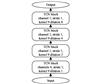 |
Fig. 5 Structure of TCN layer |
The one-dimensional convolution layer uses two-channel convolution on each time step. The kernel size is 8, and the stride is 1. The 512 hidden units of the multi-head self-attention layer are divided into 4 heads, with 21 output dimensions in the fully connected layer connected behind, which is used to classify the 21 operating states of the device. We set the respect dropout of the TCN layer, attention layer, and fully connected layer to 0.2, 0.2, and 0.1 to prevent overfitting. The negative gradient  of the LeakyReLU activation function is set to 0.1.
2.4 Lab Environment and Training Process
The hardware environments are as follows: the CPU is Intel i7-4710MQ, the GPU is NVIDIA GeForce GTX 860M GDDR5 2GB, and the RAM is DDR3L 1600MHz 8GB*2. All experiments are conducted under Windows 10 Professional Build 19041.1110 with Python 3.8 and Pytorch 1.8.1+cu102, and performed on PyCharm 2020.2 x64.
The training steps of our model are as follows:
1) Data normalization.
2) Break up the data set randomly, generate the training set and validation set from training subset with the ratio of 8:2, and convert the classification labels into one-hot vector form.
3) Initialize each layer of the model, set the optimization algorithm to Adam, the initial learning rate is 0.001 and is reduced on plateau scheduler, set the maximum number of training epochs to 50, and use cross-entropy loss function;
4) Save the model state of each epoch, and take the state with the smallest loss in the validation set as the best state.
3 Experiments and Discussion
In order to illustrate the model's diagnostic ability on multi-source time series faults, the model's performance is evaluated on the Tennessee Eastman Process (TEP) dataset.
3.1 Tennessee Eastman Process
TEP is a simulated multivariate time series dataset created by Eastman Chemical Company[32], which has nonlinear characteristics such as strong coupling and time variation[33], and is a widely used index to evaluate the model's fault diagnosis ability of complex industrial process. This simulation process is introduced by Downs et al[34] and optimized by Ricker et al[35], and consists of five components, including reactor, condenser, compressor, stripper, and separator, and provides 52 features, including 41 process measurements and 11 manipulated variables. The optimized TEP proposed by Bathelt et al[36] is shown in Fig. 6. The model has 21 operating states, including one normal state and twenty fault states, and the description of these states is shown in Table 1.
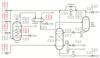 |
Fig. 6 The optimized TEP |
The standard TEP dataset can only generate limited examples for each fault, which is insufficient for training deep learning models. Therefore, we use the extended TEP dataset proposed by Rieth et al[37], who uses random seeds to generate more examples for each state. As the running state was sampled every three minutes, the training example was sampled 25 hours, i.e., 25 * 60/3 = 500 samples, and the fault state starts after an hour; the test examples were sampled 48 hours, i.e., 48 * 60/3 = 960 samples, and the fault state starts after eight hours.
In this paper, we use the training subset of raw dataset to generate the training set and validation set, the ratio of whom is 8:2, and the test set is generated from the whole test subset. The fault sampling length used in our dataset is 200, that is, the 21-220 sampling point data of the training subset is used in the training set and the validation set, and the 161-360 sampling point data of the test subset is used in the test set.
Description of TEP faults
3.2 Experiment Analysis
3.2.1 The impact of different activation functions
To demonstrate what the effect of different activation functions in TCN layer has on our model, an experiment comparing the model's performance using LeakyReLU or ReLU activation functions in TCN layer is conducted. The experiment results in Table 2 shows us the salient advantages the TCA model using the LeakyReLU activation function has over that using the ReLU activation function.
The train process of TCA model using LeakyReLU function and ReLU function is shown in Fig. 7. It is obvious that compared with the ReLU one, the model using LeakyReLU function can get more stable convergence and higher accuracy.
 |
Fig. 7 The train process of model using LeakyReLU function and ReLU function |
Accuracy and loss of TCA model using different activation functions
3.2.2 The impact of different modules in our model
In this paper, the model is improved by introducing 1DCNN and self-attention on the basis of TCN. To illustrate the validity of different module in the model, the 1DCNN and attention module are eliminated respectively to obtain four different models: TCN, TCN+Attention, TCN+1DCNN, TCA, of which the parameters in 1DCNN layer and attention layer remain unchanged, corresponding to that in TCA. All models take the epoch with the smallest loss on the validation set as the best epoch.
As shown in Table 3, the addition of 1DCNN and self-attention can enhance the ability to detect failures, improving recognition accuracy, and reducing training loss. Still, added modules will also increase epoch time. The TCA model with both 1DCNN and self-attention has the longest training time per epoch, but the highest accuracy and smallest loss.
Specifically, take the results of the above model on faults 0, 3, 9, and 15 as an example. As is shown in Fig.8, the TCN+1DCNN model has better performance on accurately detecting fault 9 comparing with the TCN model, and the TCN+Attention model can further improve the accuracy on diagnosing fault 9 but loses its accuracy on diagnosing fault 15. The proposed TCA model can combine the strengths of both TCN+1DCNN and TCN+Attention model to achieve accurate diagnosis of both types of faults simultaneously.
 |
Fig. 8 Confusion matrix of above models on fault 0, 3, 9 and 15 |
Accuracy and loss of model with different modules
3.2.3 The impact of different convolution kernels in the 1DCNN layer
To explore the performance of TCA model with different convolution kernels in the 1DCNN layer, an experiment is conducted. The kernel size of 1DCNN layer is set to 3-16, and the TCN and attention parts remain unchanged. The performance of different kernels is shown in Table 4.
From Table 4, as the kernel size increases, the training time per epoch increases as well, for a single convolution has more calculation operations, the training time increases about 29.5 s per epoch from kernel size 3 to 16. The performance of models with different kernels varies from each other; the model with kernel size 13 has the worst performance on the validation set, which is inferior to the TCN+Attention model by 0.5%. The commonly used 3 and 5-size kernels can improve the model's performance, with the accuracy being 95.07% and 94.91% respectively, which do not reach the rate of 96% and it is inferior to the model with the kernel size of 6, 8 and 16. Among all these models, the model with kernel size 8 achieves the best accuracy of 97.14%, and the best loss of 0.063.
Through the above experiments, we have explored the effects of replacing the activation function and adding 1DCNN or self-attention layer on the performance of our model. Further, the performance of the model using different convolution kernels is studied. Results in Table 2 show that the activation function replaced to LeakyReLU in TCN can effectively improve the model performance. Results in Table 3 show the effectiveness of the additional 1DCNN layer and attention layer, and the model with both the 1DCNN layer and attention layer shows the best performance. Results in Table 4 export the performance of the model with different kernel sizes in the 1DCNN layer and it is found that in most cases, the 1DCNN layer shows its effectiveness, except for that with a kernel size of 13, with the accuracy being 92.50%, which is even lower than the TCN+Attention (93.00%) model without the 1DCNN layer. The performance of other models is improved by 0.54%-4.14%, compared with the TCN+Attention model. As a result, the 1DCNN layer in our model proves its effectiveness.
Accuracy and loss of TCA model with different convolution kernels in 1DCNN layer
3.2.4 Comparison of TCA model and other neural networks
Several commonly used neural networks, including recurrent neural networks like LSTM, GRU, and Transformer, are selected to compare with our model. There are 2 or 4 layers in LSTM and GRU respectively, and the 2- or 4-layer model is marked with "2L" or "4L". Since the bidirectional RNN model might leak future samples, the RNN models here are unidirectional models. The Transformer model stacks 6 encoders. All these RNN and Transformer models have 52 dimensions in the input layer and 128 dimensions in hidden layers, and additional attention layers are added to RNN models separately, with the mark of "+A" at end, and the hidden units of these attention layers are set to 512, which are the same as those in the TCA model. To speed up the model fitting, the dropout of above models is set to 0.4. The performance of all models is shown in Table 5.
In Table 5, we can see that RNN models have natural advantages in processing time-series data; they can achieve good results with small number of parameters and short training time. Stacking more layers of RNN does not significantly enhance model's performance, but can directly lead to the training time to increase. The addition of the attention can effectively improve the model performance. As a result, the performance of RNN models with an attention layer is improved by 1.97%-4.22%. The GRU2L+A model achieves the best accuracy of 97.46% and the smallest loss of 0.057 8 on the validation set. The accuracy of Transformer model composed of encoders on the validation set achieves 92.80%, which is lower than that of the RNN models with the attention, indicating that the RNN network and the attention can complement each other.
The accuracy on the validation set of TCA model proposed in the paper achieves 97.14%, which is slightly inferior to that of the GRU2L+A model by 0.32% but surpasses those of the Transformer model and other RNN models. However, due to the extensive use of convolution, the average epoch time of the TCA model reaches 162.8 s, which is 2.78 times that of the GRU2L+A model.
Accuracy and loss of TCA model and other neural network models
3.2.5 Comparison of generalization ability of TCA and other models on the test set
An extra experiment is conducted on the test set to test the generalization ability of above models, and the widely used F1 score[38,39] is used as the evaluation indicator. Formula (7) shows the method for calculating the F1 score:
 (7)
(7)
where  , indicating the percentage of true positive samples in all positive samples tested, and
  , indicating the percentage of true positive samples in all positive samples.
The F1 score, accuracy, and loss of the above models on the test set are shown in Table 6.
As shown in Table 6, among all the 21 faults, our TCA model achieves the best accuracy of 94.27%, loss of 0.331 9 and the average F1 score of 0.9405 on the test set, and achieves the best F1 score on 16 faults across all 21 faults. Among the most difficult faults 3, 9 and 15, the respect F1 score of TCA also achieves 0.752 8, 0.900 7, and 0.769 7, which is the best F1 score for faults 9 and 15. The confusion matrix in Fig. 9 shows the detailed result clearly that our model can accurately identify most faults, especially for fault 9 and 15, whose accuracy reaches 93% and 71%, respectively. Although the GRU2L+A model performs better than the TCA model on validation set, its generalization ability is slightly worse than that of the TCA model on the test set. In all 21 faults, the F1 score of the TCA model is not inferior to that of GRU2L+A model for 20 faults, and is superior to that for 9 faults, but substantially inferior to that for fault 5. The confusion matrix can show the identification result of fault 5 clearly, though accurately our model can identify fault 5, the misidentification of large numbers of fault 3 samples as fault 5 results in a low F1 score of it. Meanwhile, the matrix shows that the recognition ability of our model between fault 0 (normal state) and fault 15 still needs to be strengthened; about 27% fault 0 states are recognized as fault 15 and 14% fault 15 as fault 0, demonstrating the main reason of accuracy loss; 29% fault 5 as fault 3 is another cause. However, our model still achieves the best F1 score of 0.661 4 on fault 0, indicating the most robust discrimination ability under a normal state and fault condition.In addition, the model is tested on the partner's diesel engine failure dataset, on which project this paper relies. Failures such as reduced compressor efficiency, extended combustion duration and reduced fuel injection of diesel engines can lead to a slow decrease in the output power of diesel engine and aggravate the wear of diesel engine parts, which reduces the operational stability. We use the collected time-series sensors data as model input. The results turn out that the model can quickly and effectively detect faults compared with the manual detection method.
 |
Fig. 9 Confusion matrix of TCA on the test set |
F1 score, total accuracy and loss of the models on the test set
4 Conclusion
For complex multivariate industrial process faults that are strongly coupled and time-varying, a TCA model based on TCN together with 1DCNN and multi-head self-attention is proposed, and we further improve the model by replacing the activation function of TCN. The introduction of 1DCNN can effectively extract the local correlations of multivariate, and the following multi-head self-attention can automatically assign higher weights to important features. The experiment results validates its effectiveness.
References
- Wu D, Ren G, Wang H, et al. The review of mechanical fault diagnosis methods based on convolutional neural network [J]. Journal of Mechanical Strength, 2020, 42(5): 1024-1032(Ch). [Google Scholar]
- Zhang Y, Zhang L L. Intelligent fault detection of reciprocating compressor using a novel discrete state space [J]. Mechanical Systems and Signal Processing, 2022, 169: 108583. [NASA ADS] [CrossRef] [Google Scholar]
- Pulido B, Zamarreno J M, Merino A, et al. State space neural networks and model-decomposition methods for fault diagnosis of complex industrial systems [J]. Engineering Applications of Artificial Intelligence, 2019, 79: 67-86. [CrossRef] [Google Scholar]
- Sakar C, Toz A C, Buber M, et al. Risk analysis of grounding accidents by mapping a fault tree into a Bayesian network [J]. Applied Ocean Research, 2021, 113(1): 1-12. [Google Scholar]
- Tan Q, Mu X W, Fu M, et al. A new sensor fault diagnosis method for gas leakage monitoring based on the naive Bayes and probabilistic neural network method [J]. Measurement, 2022, 194: 111037. [Google Scholar]
- Farshad M. Detection and classification of internal faults in bipolar HVDC transmission lines based on K-means data description method [J]. International Journal of Electrical Power & Energy Systems, 2019, 104: 615-625. [CrossRef] [Google Scholar]
- Chen G C, Liu Y, Ge Z Q. K-means Bayes algorithm for imbalanced fault classification and big data application [J]. J Process Control, 2019, 81: 54-64. [CrossRef] [Google Scholar]
- Yu Y, Peng M, Wang H J, et al. Improved PCA model for multiple fault detection, isolation and reconstruction of sensors in nuclear power plant [J]. Ann Nucl Energy, 2020, 148: 107662. [CrossRef] [Google Scholar]
- Li G N, Hu Y P. An enhanced PCA-based chiller sensor fault detection method using ensemble empirical mode decomposition based denoising [J]. Energy & Buildings, 2019, 183: 311-324. [CrossRef] [Google Scholar]
- Krizhevsky A, Sutskever I, Hinton G E. Imagenet classification with deep convolutional neural networks[C]// Advances in Neural Information Processing Systems. New York: Curran Associates Inc, 2012: 1097-1105. [Google Scholar]
- Cho K, Merrienboer B V, Gulcehre C, et al. Learning phrase representations using RNN encoder-decoder for statistical machine translation[C]// Proceedings of the 2014 Conference on Empirical Methods in Natural Language Processing. Stroudsburg: ACL, 2014: 1724-1734. [Google Scholar]
- He K M, Zhang X Y, Ren S Q, et al. Deep residual learning for image recognition[C]// 2016 IEEE Conference on Computer Vision and Pattern Recognition (CVPR). Piscataway: IEEE, 2016: 770-778. [Google Scholar]
- Vaswani A, Shazeer N, Parmar N, et al. Attention is all you need[C]// Advances in Neural Information Processing Systems. Cambridge: MIT Press, 2017: 5998-6008. [Google Scholar]
- Devlin J, Chang M W, Lee K, et al. BERT: Pre-training of deep bidirectional transformers for language understanding[EB/OL]. [2022-06-17]. https://arxiv.org/pdf/1810.04805.pdf. [Google Scholar]
- Hu J , Shen L, Albanie S, et al. Squeeze-and-excitation networks [J]. IEEE Transactions on Pattern Analysis and Machine Intelligence, 2020, 42(8): 2011-2023. [CrossRef] [PubMed] [Google Scholar]
- Asgari S, Gupta R, Puri I K, et al. A data-driven approach to simultaneous fault detection and diagnosis in data centers [J]. Applied Soft Computing, 2021, 110: 107638. [CrossRef] [Google Scholar]
- Chen Y J, Rao M, Feng K, et al. Physics-Informed LSTM hyperparameters selection for gearbox fault detection [J]. Mechanical Systems and Signal Processing, 2022, 171: 108907. [Google Scholar]
- Li J Q, Liu J, Chen Y T. A fault warning for inter-turn short circuit of excitation winding of synchronous generator based on GRU-CNN [J]. Global Energy Interconnection, 2022, 5(2): 236-248. [CrossRef] [Google Scholar]
- Rehmer A, Kroll A. On the vanishing and exploding gradient problem in Gated Recurrent Units [J]. IFAC-PapersOnLine, 2020, 53(2): 1243-1248. [CrossRef] [Google Scholar]
- Sak H, Senior A, Beaufays F. Long short-term memory based recurrent neural network architectures for large vocabulary speech recognition[EB/OL]. [2022-06-17]. https://arxiv.org/pdf/1402.1128.pdf. [Google Scholar]
- Kang S H, Han J H. New RNN activation technique for deeper networks: LSTCM cells [J]. IEEE Access, 2020, 8:214625-214632. [CrossRef] [Google Scholar]
- Wu H , Zhao J S. Deep convolutional neural network model based chemical process fault diagnosis [J]. Comput Chem Eng, 2018, 115: 185-197. [CrossRef] [Google Scholar]
- Song Q S, Jiang P. A multi-scale convolutional neural network based fault diagnosis model for complex chemical [J]. Process Saf Environ Prot, 2022, 159: 575-584. [CrossRef] [Google Scholar]
- Deng L, Zhang Y, Dai Y Y, et al. Integrating feature optimization using a dynamic convolutional neural network for chemical process supervised fault classification [J]. Process Safety and Environmental Protection, 2021, 155: 473-485. [CrossRef] [Google Scholar]
- Bai S, Kolter J Z, Koltun V. An empirical evaluation of generic convolutional and recurrent networks for sequence modeling[EB/OL]. [2022-06-17]. https://arxiv.org/pdf/1803.01271. [Google Scholar]
- Waibel A, Hanazawa T, Hinton G E, et al. Phoneme recognition using time-delay neural networks [J]. Readings in Speech Recognition, 1990, 1(3): 393-404. [CrossRef] [Google Scholar]
- Ji W, Chee K C. Prediction of hourly solar radiation using a novel hybrid model of ARMA and TDNN [J]. Solar Energy, 2011, 85(5): 808-817. [NASA ADS] [CrossRef] [Google Scholar]
- Tang W P, Wang A Q, Ramkumar S, et al. Signal identification system for developing rehabilitative device using deep learning algorithms [J]. Artificial Intelligence in Medicine, 2020, 102: 101755. [CrossRef] [PubMed] [Google Scholar]
- Zhang X B, Xu X G, Zhu Y X. An improved time delay neural network model for predicting dynamic heat and mass transfer characteristics of a packed liquid desiccant dehumidifier [J]. Int J Therm Sci, 2022, 177: 107548. [CrossRef] [Google Scholar]
- Liang H P, Zhao X Q. Rolling bearing fault diagnosis based on one-dimensional dilated convolution network with residual connection[J]. IEEE Access, 2021, 9: 31078-31091. [CrossRef] [Google Scholar]
- Xia J, Feng Y W, Teng D, et al. Distance self-attention network method for remaining useful life estimation of aeroengine with parallel computing [J]. Reliability Engineering & System Safety, 2022, 225: 108636. [CrossRef] [Google Scholar]
- Reinartz C, Kulahci M, Ravn O. An extended Tennessee Eastman simulation dataset for fault-detection and decision support systems [J]. Comput Chem Eng, 2021, 149: 107281. [CrossRef] [Google Scholar]
- Yin S, Ding S X, Haghani A, et al. A comparison study of basic data-driven fault diagnosis and process monitoring methods on the benchmark Tennessee Eastman process [J]. J Process Control, 2012, 22(9): 1567-1581. [CrossRef] [Google Scholar]
- Downs J J, Vogel E F. A plant-wide industrial process control problem [J]. Comput Chem Eng, 1993, 17(3): 245-255. [CrossRef] [Google Scholar]
- Ricker N L. Optimal steady-state operation of the Tennessee Eastman challenge process [J]. Comput Chem Eng, 1995, 19(9): 949-959. [CrossRef] [Google Scholar]
- Bathelt A, Ricker N L, Jelali M. Revision of the Tennessee Eastman process model[J]. IFAC PapersOnLine, 2015, 48(8): 309-314. [CrossRef] [Google Scholar]
- Rieth C A, Amsel B D, Tran R, et al. Issues and advances in anomaly detection evaluation for joint human-automated systems[C]// International Conference on Applied Human Factors and Ergonomics. Berlin: Springer-Verlag, 2017: 52-63. [Google Scholar]
- Xu Y, Cong K D, Zhu Q X, et al. A novel AdaBoost ensemble model based on the reconstruction of local tangent space alignment and its application to multiple faults recognition [J]. J Process Control, 2021, 104(3): 158-167. [CrossRef] [Google Scholar]
- Yu W B, Lv P. An end-to-end intelligent fault diagnosis application for rolling bearing based on MobileNet [J]. IEEE Access, 2021, 9: 41925-41933. □ [CrossRef] [Google Scholar]
All Tables
All Figures
|
Fig. 1 Dilated convolution |
| In the text | |
|
Fig. 2 The residual connection of TCN |
| In the text | |
|
Fig. 3 Network structure |
| In the text | |
|
Fig. 4 Overall train process |
| In the text | |
|
Fig. 5 Structure of TCN layer |
| In the text | |
|
Fig. 6 The optimized TEP |
| In the text | |
|
Fig. 7 The train process of model using LeakyReLU function and ReLU function |
| In the text | |
|
Fig. 8 Confusion matrix of above models on fault 0, 3, 9 and 15 |
| In the text | |
|
Fig. 9 Confusion matrix of TCA on the test set |
| In the text | |
Current usage metrics show cumulative count of Article Views (full-text article views including HTML views, PDF and ePub downloads, according to the available data) and Abstracts Views on Vision4Press platform.
Data correspond to usage on the plateform after 2015. The current usage metrics is available 48-96 hours after online publication and is updated daily on week days.
Initial download of the metrics may take a while.