| Issue |
Wuhan Univ. J. Nat. Sci.
Volume 30, Number 2, April 2025
|
|
|---|---|---|
| Page(s) | 139 - 149 | |
| DOI | https://doi.org/10.1051/wujns/2025302139 | |
| Published online | 16 May 2025 | |
Mathematics
CLC number: O241
Numerical Integration of the Function with Twin Boundary Layers
带有双边界层函数的数值积分
School of Mathematical Sciences, Suzhou University of Science and Technology, Suzhou 215009, Jiangsu, China
† Corresponding author. E-mail: This email address is being protected from spambots. You need JavaScript enabled to view it.
Received:
28
May
2024
Abstract
Traditional numerical integration requires sufficient smoothness of the integrand to achieve high-order algebraic accuracy. If the function has a boundary layer with large gradient, the composite integration formula on the uniform mesh will produce very large integration errors. In this paper, we study the Newton-Cotes formula based on Lagrange interpolation functions, local  projection approximating the integrand, and Gauss integration. On the Shishkin mesh, we establish an optimal-order integration error estimate uniformly in the perturbation parameter. The convergence rate is the same as that for the smooth function. Numerical experiments confirm the sharpness of our theoretical results.
摘要
传统的数值积分需要被积函数具有较高的光滑性以获得高阶代数精度。当函数具有大梯度变化的双边界层时,基于均匀网格的复化积分公式将产生较大的积分误差。本文研究三类数值积分公式,即基于拉格朗日基函数的牛顿-科特斯公式、被积函数基于局部L2投影近似以及经典的高斯积分。借助于分片一致的Shishkin网格,证明了与小参数无关的最优阶积分误差估计,该收敛阶与光滑函数数值积分收敛阶相同。数值实验证实了我们的理论结果。
Key words: boundary layers / Shishkin mesh / Newton-Cotes formula / local L2 projection / Gauss integration
关键字 : 边界层 / Shishkin网格 / 牛顿-科特斯公式 / 局部L2-投影 / 高斯积分
Cite this article: KANG Juan, CHENG Yao. Numerical Integration of the Function with Twin Boundary Layers[J]. Wuhan Univ J of Nat Sci, 2025, 30(2): 139-149.
Biography: KANG Juan, female, Master candidate, research direction: numerical analysis of the differential equations. E-mail: This email address is being protected from spambots. You need JavaScript enabled to view it.
Foundation item: Supported by the National Natural Science Foundation of China (11801396), Natural Science Foundation of Jiangsu Province (BK20170374), Qing Lan Project of Jiangsu University and Graduate Student Scientific Research Innovation Projects of Jiangsu Province (KYCX24_3407)
© Wuhan University 2025
 This is an Open Access article distributed under the terms of the Creative Commons Attribution License (https://creativecommons.org/licenses/by/4.0), which permits unrestricted use, distribution, and reproduction in any medium, provided the original work is properly cited.
0 Introduction
The definite integration plays an important role in calculus. It is usually calculated by the well-known Newton-Leibniz formula. However, when the integrand cannot be represented by fundamental functions, the primitive function is complicated or the integrand has no analytic expression (e.g., some discrete point values are known), numerical integration becomes a practical necessity.
To date, the common numerical integrations are based on the composite Newton-Cotes formula. If the integrand is sufficiently smooth, the error of the composite trapezoidal and Simpson rule can attain  and
and  , where
  is the cell size. Otherwise, the composite Newton-Cotes formula based on the uniform mesh will produce very large errors.
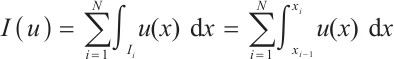
Consider the numerical approximation for the following definite integration
 (1)
(1)
Assume that the function  can be decomposed as
 (2)
(2)
where  is the regular component,
  and
and  are the two boundary layer components, which satisfy
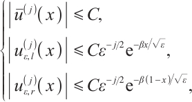 (3)
(3)
for any  where
where  is a small positive parameter,
  is a given positive constant and
  is an integer. It is obvious that the function
  exhibits a typical boundary layer, namely it has large gradients at the boundary ends
  and
and  .
.
Such function of (2) can be viewed as the solution of the singularly perturbed reaction-diffusion problem
 (4)
(4)
where 
 and
and  are smooth functions. The problem (4) has wide applications in such fields as optimal control, chemical reactions, fluid dynamics and so on. It is of great scientific significance to study the corresponding numerical solutions[1].
Regarding the solution to the singularly perturbed convection-diffusion problem, there are abundant results on the numerical integration. For example, it was shown in Refs. [2-3] that the composite trapezoidal and Simpson rule on the uniform mesh will lead to an integration error of order  . Ref. [4] studied the Lagrange interpolation of piecewise polynomials of degree
  and the composite Newton-Cotes formula on a piecewise-uniform Shishkin mesh[5]. The convergence rate is
  , where
  is the number of total elements. In Ref. [6], the results were extended to the Bakhvalov mesh[7-8], the interpolation error was proved to be
  and the integration error was
  . Furthermore, a new
  point interpolation formula was discussed in Ref. [9]. The interpolation error was proved to be
  when
when  , but increased to
  if
if  is small. Ref. [10] showed the error of the Gauss integral formula using
  nodes on the Shishkin mesh, the convergence rate is
  .
.
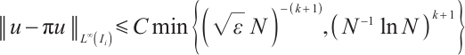
However, all the above results were obtained for the integrand with one-sided boundary layer. There are very few results on the numerical integration for the solution of the singularly perturbed reaction-diffusion problem (4) with twin boundary layers. In this paper, we address this problem and present three types of numerical integrations on the Shishkin mesh. We derive some error estimates that are uniform in the perturbation parameter  . The contributions of this paper are the following:
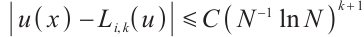
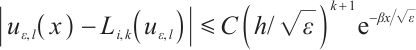
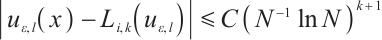
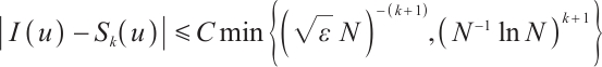
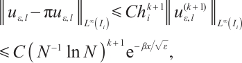
1) We prove that the Lagrange interpolation on the Shishkin mesh converges at a rate of order 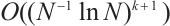 , when piecewise polynomials of degree
  and total element number
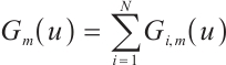
  are used. Consequently, we obtain an integral error
  for the Newton-Cotes formula on the Shishkin mesh, see Theorems 1 and 2.
2) Based on the local  projection for the integrand, we obtain an integral error of order
  , see Theorems 3 and 4.
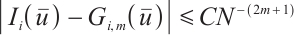
3) We prove that the Gauss integral formula using  nodes on the Shishkin mesh can attain a convergence order
  , see Theorem 5.
1 Shishkin Mesh
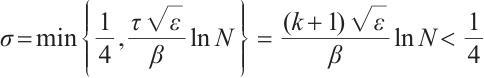
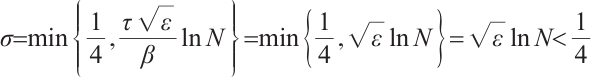
Define the mesh transition parameter
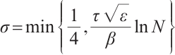 (5)
(5)
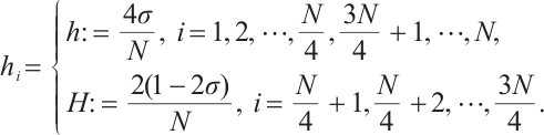
where  is a user-chosen parameter whose value will be discussed later. The mesh points are given by
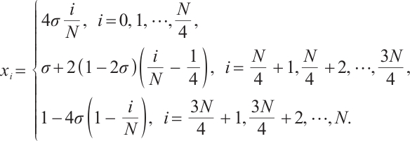
Set the Shishkin mesh as  with element
  . Set the mesh size
  and then we have
 (6)
(6)
Denote 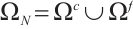 , where
 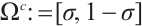 is the coarse domain and
  is the refined domain. Figure 1 shows a Shishkin mesh for
  .
.
 |
Fig. 1 The Shishkin mesh ( ) )
|
2 The Newton-Cotes Formula and Its Error Estimate
The common numerical integration is based on the Newton-Cotes formula using the Lagrange interpolation for the integrand. However, for the function (2) with boundary layer, the traditional method on the uniform mesh will result in a large error. This section presents the Lagrange interpolation and the Newton-Cotes formula on the Shishkin mesh. We will establish optimal-order error estimates that are independent of the small parameter  .
.
2.1 The Lagrange Interpolation
Assume that  is a multiple of
  , and divide the domain
  into
into  subintervals
where  represents the set of cell
 . On each interval
  , we define the Lagrange interpolation of
  by
by
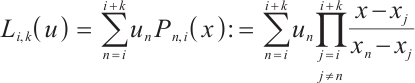 (7)
(7)
where  is the base function with degree k.
Define the Lebesgue constant of  as
as
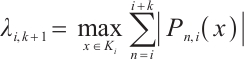 (8)
(8)
Since  is a multiple of
  , we have
  or
or  . Therefore, the subinterval
  is uniform. From Ref. [11], one has
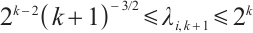 (9)
(9)
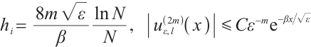
Lemma 1 Let  be the mesh size of the interval
  . Denote
  , then one has
 (10)
(10)
Proof Without loss of generality, let  . For any
  one has
  and
and
thus  .
.
This finishes the proof.
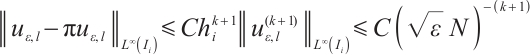
2.2 Error Estimate of the Lagrange Interpolation
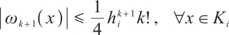
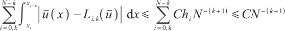
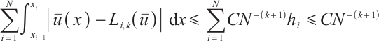
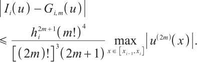
Lemma 2 One has the following interpolation error
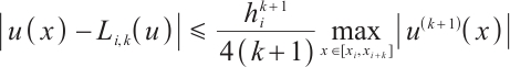 (11)
(11)
Proof From Ref. [12], one has
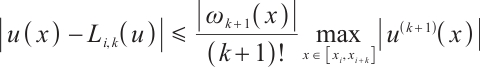 (12)
(12)
Then (11) follows from Lemma 1.
Theorem 1 Suppose that  satisfies (2) and (3) and set
  . Then one has the following interpolation error estimates.
If  and
and 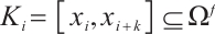 , then
 (13)
(13)
If  and
and  , then
 (14)
(14)
If  , then
 (15)
(15)
Here the bounding constant  is independent of
  and
and  .
.
Proof From (3) and (11), one has
then
 (16)
(16)
To bound the interpolation error for the left boundary layer component  we proceed from the following two situations.
Case 1 
For  , it follows from (3) and (6) that
 (17)
(17)
Noticing
 (18)
(18)
and Lemma 2, one obtains
 (19)
(19)
namely,
 (20)
(20)
For  , due to (3) and
  , one obtains
 (21)
(21)
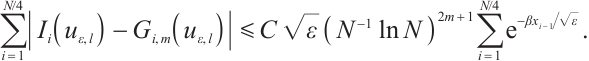
From (7), (8) and (21), one gets
Hence
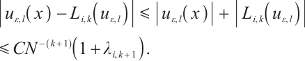
Using (9) yields
 (22)
(22)
Case 2 
The partition  is uniform and
  . By (11), one has

If  , then
In a similar manner, one can bound the interpolation error for the right boundary layer component  . This finishes the proof.
2.3 Error Estimate of the Newton-Cotes Formula
Let
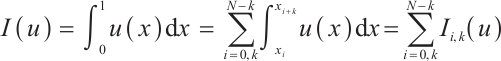 (23)
(23)
where  satisfies (2) and (3). On the Shishkin mesh
  with
with  , we introduce the Newton-Cotes formula with
  nodes
nodes
 (24)
(24)
Theorem 2 Suppose that  satisfies (2) and (3) and set
  . Then one has the following integral error estimates.
If  , then
 (25)
(25)
If  , then
 (26)
(26)
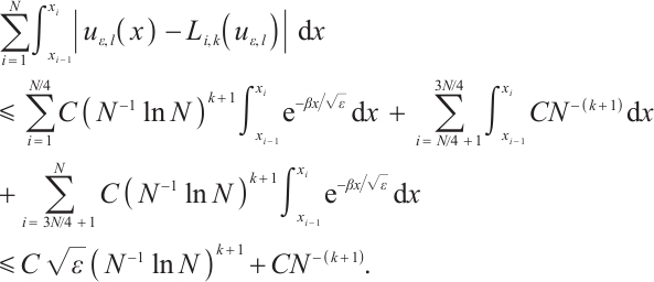
Proof We proceed from the following two situations.
Case 1 
Now one has 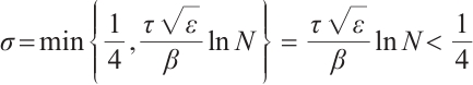 .
.
By (16), one has
Using (19) and (22) yields
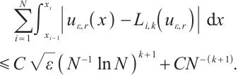
Analogously,
Collecting the above estimates gives
 (27)
(27)
Case 2 
Now one has 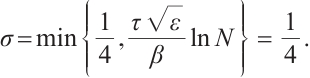
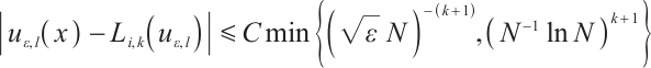
Using (15), one obtains
 (28)
(28)
This finishes the proof.
3 Numerical Integration Based on Local  Projection
It is common to use the projection polynomials to approximate the integrand. Local  projection can realize element orthogonality and is widely used in the approximation theory and finite element error analyses. In this section, we discuss the numerical integration using the local
  projection for the integrand.
3.1 Local  Projection
Let  be the space composed with piecewise degree of at most
  on the subinterval
  . For any
  , define
  by
by
Denote  by the usual maximum-norm on the cell
  . We have the following projection error estimates on the Shishkin mesh.
Lemma 3[13] There exists a constant  independent of
  and
and  such that
 (29)
(29)
 (30)
(30)
3.2 Error Estimate
Theorem 3 Suppose that  satisfies (2) and (3) and set
  . Then one has the following projection error estimates.
If  and
and  , then
 (31)
(31)
If  and
and  , then
 (32)
(32)
If  , then
 (33)
(33)
Here the bounding constant  is independent of
  and
and  .
.
Proof Recall 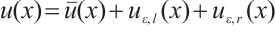 . From (3) and (29), one has
 (34)
(34)
Now we turn to bound the projection error for the left boundary layer component  .
.
Case 1 
For  , it follows from (17) and (29) that
 (35)
(35)
namely,
 (36)
(36)
For  , the inequalities (21), (30) and
  give
give
 (37)
(37)
Case 2 
The partition  is uniform and
  . By (11), one has
Note that  implies
  , then one gets
 (38)
(38)
In a similar manner, one can bound the projection error for the right boundary layer component  . This finishes the proof.
Theorem 4 Define 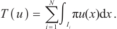 Suppose that
  satisfies (2) and (3) and set
  . Then one has the following integral error estimates.
If 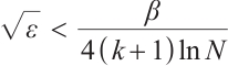 , then
 (39)
(39)
If , then
 (40)
(40)
Proof We proceed from the following two situations.
Case 1 
Now one has
From (34), one obtains
From (35) and (37), one has
Likewise, one gets
Collecting the above estimates gives
 (41)
(41)
Case 2 
Now one has  It follows from (33) that
 (42)
(42)
This finishes the proof.
4 Gauss Integration and Its Error Estimate
Gauss integration has the highest algebraic accuracy with the same number of interpolation nodes, and is favored by numerical analysts in the practical computation. In this section, we consider the Gauss integration formula on the Shishkin mesh and derive some uniform error estimates.
4.1 Gauss Integration
Define the Gauss integration formula with  nodes for the element
  ,
,
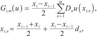 (43)
(43)
where  is the Gauss weight and
  is the root of the Legendre polynomial of degree
  in the interval
  . Consider the Gauss formula
 (44)
(44)
which approximates
 (45)
(45)
In the following we assume that  in the inequality (3) and
  in (5).
4.2 Error Estimate of the Gauss Integration
Lemma 4[14] Let  be the mesh size of element
  , then one has the following error estimate
 (46)
(46)
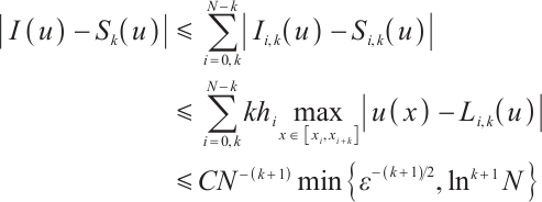
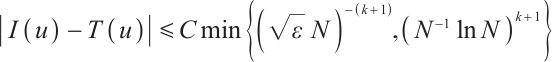
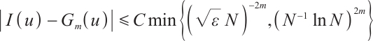
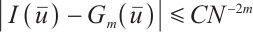
Theorem 5 Suppose that  satisfies (2) and (3). Then one has the following integral error estimates.
If  , then
 (47)
(47)
If  , then
 (48)
(48)
Proof Due to  and Lemma 4, one has
namely,
 (49)
(49)
Now we deal with the integration error of  .
.
Case 1 
Note that  , one has
For  , due to (3), one gets
 (50)
(50)
By Lemma 4, one has
 (51)
(51)
hence
The geometric series gives
due to  .
.
Then, one has
For  , the inequality (3) gives
 (52)
(52)
Since  and
and  due to (43), so one has
 (53)
(53)
Combining (52) and (53) yields
Case 2 
Now one has  . By (3) and (46), one has
Since  , one obtains
 (54)
(54)
Similarly, one can obtain the integration error for  . This proves Theorem 5.
5 Numerical Experiments
Consider a function
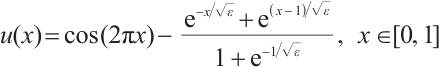 (55)
(55)
which exhibits twin boundary layers at  and
and  , see Fig. 2.
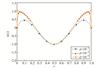 |
Fig. 2 A function with twin boundary layers |
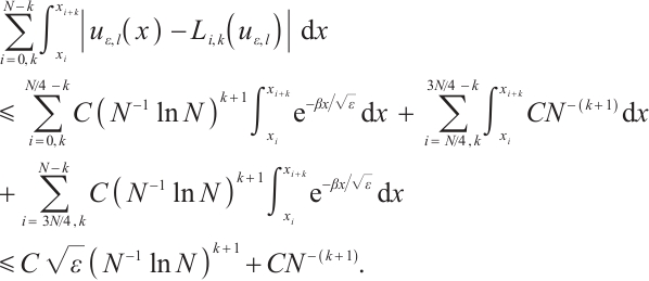
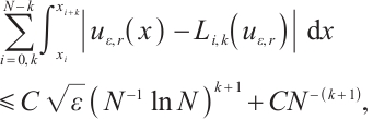
In this section, we present the numerical results for the composite Newton-Cotes formula, piecewise discontinuous  projection and Gauss integration formula on the Shishkin mesh. Set
  for the former two cases and
  for the last case.
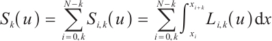
5.1 Newton-Cotes Formula
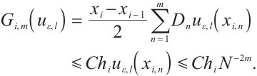
Consider the composite Newton-Cotes formula with four points
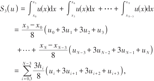
where  is the cell size of the interval
  and the notation
  refers to the summation calculated from
  . Given
  and
and  , we define the integration error as
  . The convergence order is computed by
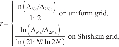
because it shall behave as  and
and  for uniform and Shishkin meshes, respectively.
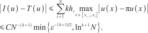
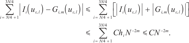
Table 1 shows the error and convergence rate of the integration formula  on the uniform mesh. The convergence order is generally
  . However, when
  the convergence order deteriorates significantly. On the Shishkin mesh, the convergence order is restored. Table 2 shows that the convergence rate of the integration error is always
  . This is fully consistent with Theorem 2.
Integration error and convergence rate using Newton-Cotes formula on the uniform mesh ( )
)
Integration error and convergence rate using Newton-Cotes formula on the Shishkin mesh ( )
)
5.2 Local  Projection
Consider the local  projection into the space of the piecewise cubic polynomials, namely
  , the projection error is defined as
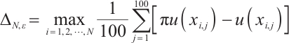
Table 3 shows the projection error on the uniform mesh. When  is large, the convergence order attains
  , but as
  decreases to zero, the convergence order deteriorates sharply. On the Shishkin mesh, the rate of convergence is robust and remains
  , as shown in Table 4. This agrees with our prediction in Theorem 3.
 projection error and convergence rate on the uniform mesh
 projection error and convergence rate on the Shishkin mesh
5.3 Gauss Integration
Consider the composite Gauss integration formula with three nodes, namely  ,
,
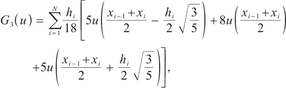
where  . Given
  and
and  , define integration error as
  .
.
Table 5 shows the integration error and its convergence rate on the uniform mesh. When  is large, the rate of convergence attains
  . However, as
  becomes smaller, the convergence rate deteriorates quickly. On the Shishkin mesh, the convergence rate is improved, and is always
  , see Table 6. This is fully consistent with Theorem 5.
Integration error and convergence rate using Gauss formula on the uniform mesh
Integration error and convergence rate using Gauss formula on the Shishkin mesh
6 Conclusion
We discussed the numerical integration of the function with large gradients. The traditional numerical integration on the uniform mesh produces very large errors. We present three numerical integrations on the Shishkin mesh, i.e., the Newton-Cotes formula, local  projection and Gauss integration. We derive an optimal-order error estimate independent of the small perturbation parameter. Numerical experiments confirm the sharpness of our theoretical findings. In future work, we would like to extend the results to the other types of layer-adapted meshes, such as Bakhvalov-type meshes and graded meshes[15].
References
- Roos H G, Stynes M, Tobiska L. Robust Numerical Methods for Singularly Perturbed Differential Equations[M]. 2nd Edition. Berlin: Springer-Verlag, 2008. [Google Scholar]
- Zadorin A I, Zadorin N A. Quadrature formulas for functions with a boundary-layer component[J]. Computational Mathematics and Mathematical Physics, 2011, 51(11): 1837-1846. [Google Scholar]
- Zadorin A I. New approaches to constructing quadrature formulas for functions with large gradients[J]. Journal of Physics: Conference Series, 2021, 1901(1): 012055. [Google Scholar]
- Zadorin A I. Lagrange interpolation and Newton-Cotes formulas for functions with boundary layer components on piecewise-uniform grids[J]. Numerical Analysis and Applications, 2015, 8(3): 235-247. [Google Scholar]
- Shishkin G I. Grid approximations of singularly perturbed elliptic equations in domains with characteristic faces[J]. Russian Journal of Numerical Analysis and Mathematical Modelling, 1990, 5: 327-344. [Google Scholar]
- Zadorin A I, Zadorin N A. Lagrange interpolation and the Newton-Cotes formulas on a Bakhvalov mesh in the presence of a boundary layer[J]. Computational Mathematics and Mathematical Physics, 2022, 62(3): 347-358. [Google Scholar]
- Bakhvalov N S. The optimization of methods of solving boundary value problems with a boundary layer[J]. USSR Computational Mathematics and Mathematical Physics, 1969, 9(4): 139-166. [Google Scholar]
- Linß T. Layer-Adapted Meshes for Reaction-Convection-Diffusion Problems[M]. Berlin: Springer-Verlag, 2010. [Google Scholar]
- Zadorin A I, Zadorin N A. Interpolation formula for functions with a boundary layer component and its application to derivatives calculation[J]. Siberian Electronic Mathematical Reports, 2012, 9: 445-455. [Google Scholar]
- Zadorin A I. Gauss quadrature on a piecewise uniform mesh for functions with large gradients in a boundary layer[J]. Siberian Electronic Mathematical Reports, 2016, 13: 101-110. [Google Scholar]
- Kornev A A, Chizhonkov E V. Uprazhneniya po chislennym metodam[M]. Moscow: Moscow State Univ, 2003: 26. [Google Scholar]
- Sun Z Z, Wu H W. An Elementary Numerical Analysis[M]. 5th Edition. Nanjing: Southeast University Press, 2011: 89(Ch). [Google Scholar]
- Brenner S C, Scott L R. The Mathematical Theory of Finite Element Methods[M]. New York: Springer-Verlag, 2002. [Google Scholar]
- Jiang E X, Zhao F G. Numerical Approximation[M]. 2nd Edition. Shanghai: Fudan University Press, 2008: 160(Ch). [Google Scholar]
- Durán R G, Lombardi A L. Finite element approximation of convection diffusion problems using graded meshes[J]. Applied Numerical Mathematics, 2006, 56(10/11): 1314-1325. [Google Scholar]
All Tables
Integration error and convergence rate using Newton-Cotes formula on the uniform mesh ()
Integration error and convergence rate using Newton-Cotes formula on the Shishkin mesh ()
All Figures
|
Fig. 1 The Shishkin mesh ()
|
| In the text | |
|
Fig. 2 A function with twin boundary layers |
| In the text | |
Current usage metrics show cumulative count of Article Views (full-text article views including HTML views, PDF and ePub downloads, according to the available data) and Abstracts Views on Vision4Press platform.
Data correspond to usage on the plateform after 2015. The current usage metrics is available 48-96 hours after online publication and is updated daily on week days.
Initial download of the metrics may take a while.