On Numerical Examples of Boundary Knot Method for Helmholtz-Type Equation

Peilan MA; Nan MENG

doi:10.1051/wujns/2025303283

All issues

Volume 30 / No 3 (June 2025)

Wuhan Univ. J. Nat. Sci., 30 3 (2025) 283-288

Full HTML

Open Access

Issue		Wuhan Univ. J. Nat. Sci. Volume 30, Number 3, June 2025


Page(s)		283 - 288
DOI		https://doi.org/10.1051/wujns/2025303283
Published online		16 July 2025

Wuhan University Journal of Natural Sciences, 2025, Vol.30 No.3, 283-288

Mathematics

CLC number: O242

On Numerical Examples of Boundary Knot Method for Helmholtz-Type Equation

边界节点法求解Helmholtz型方程的数值算例研究

Peilan MA (马培兰) and Nan MENG (孟楠)

General Education Center, Zhengzhou Business University, Zhengzhou 451200, Henan, China

Received: 15 December 2024

Abstract

The boundary knot method (BKM) is a simple boundary-type meshless method. Due to the use of non-singular general solutions rather than singular fundamental solutions, BKM does not need to consider the artificial boundary. Therefore, this method has the merits of purely meshless, easy to program, high solution accuracy and so on. In this paper, we investigate the effectiveness of the BKM for solving Helmholtz-type problems under various conditions through a series of novel numerical experiments. The results demonstrate that the BKM is efficient and achieves high computational accuracy for problems with smooth or continuous boundary conditions. However, when applied to discontinuous boundary problems, the method exhibits significant numerical instability, potentially leading to substantial deviations in the computed results. Finally, three potential improvement strategies are proposed to mitigate this limitation.

摘要

边界节点法是一种简单的边界型无网格方法。由于采用非奇异通解而不是奇异基本解，无需考虑人工边界的问题，因此边界节点法具有纯无网格、易于编程、求解精度高等优点。本文通过一系列新的数值实验，研究了边界节点法在不同条件下求解Helmholtz型问题的有效性。研究结果表明，对于具有光滑或连续边界条件的问题，边界节点法有效且具有较高的计算精度。然而，在处理不连续边界问题时，该方法存在明显的数值不稳定性，计算结果可能出现显著偏差。最后，针对这一局限性，提出了三个可能的改进方向。

Key words: boundary knot method / meshless method / non-singular general solution, Helmholtz-type equation

关键字 : 边界节点法 / 无网格方法 / 非奇异通解 / Helmholtz型方程

Cite this article: MA Peilan, MENG Nan. On Numerical Examples of Boundary Knot Method for Helmholtz-Type Equation[J]. Wuhan Univ J of Nat Sci, 2025, 30(3): 283-288.

Biography: MA Peilan, female, Associate professor, research direction: computational mathematics. E-mail: mapeilan1987@126.com

Foundation item: Supported by the Key Scientific Research Plan of Colleges and Universities in Henan Province (23B140006)

© Wuhan University 2025

This is an Open Access article distributed under the terms of the Creative Commons Attribution License (https://creativecommons.org/licenses/by/4.0), which permits unrestricted use, distribution, and reproduction in any medium, provided the original work is properly cited.

0 Introduction

In recent years, meshless methods have made significant progress in the field of computational mechanics and engineering applications, gradually evolving into an important numerical tool for handling complex scientific computing problems. The Meshless Local Petrov-Galerkin (MLPG) method^[1-2] has attracted considerable attention in the academic community due to its unique theoretical advantages and has demonstrated excellent numerical performance in computational solid mechanics, fracture mechanics, and multiphysics coupling analysis. Interpolation methods based on Radial Basis Functions (RBF)^[3-4] have gradually become an important branch of meshless methods research, thanks to their unique advantages in dealing with irregular geometric boundaries and high-dimensional space problems, providing new solutions for the numerical simulation of complex engineering problems. Recently, a novel meshless backward substitution method (BSM)^[5-6] has been proposed to address multi-point problems and time-dependent issues.

As is known to all, meshless methods are mature in dealing with many boundary value problems, as demonstrated in recent studies^[7-10]. One of the popular boundary-type meshless collocation methods, which was named the boundary knot method (BKM), was pioneered by Kang and his coworkers^[11].

The BKM has been applied to many problems, including two-dimensional^[12], three-dimensional^[13] and inverse problems^[14-15]. For the traditional ill-conditioned interpolation matrix, the effective condition number is introduced to scale the BKM^[16], and some regularization methods^[17] are considered in dealing with direct problems by using the BKM. An early work made an overview of this method^[18], and it proposed three new BKM methods and discussed their problems in solving the Helmholtz equation and future research directions.

In previous academic literatures, it is generally believed that the BKM can provide high-precision numerical solutions for transient heat conduction^[19], convection-diffusion problems^[20], acoustic problems^[21] and Helmholtz-type equations^[22]. However, these studies often focused on ideal boundary conditions, assuming that the Dirichlet and Neumann boundary conditions are smooth^{[13, 23-24]}. This assumption raises a question that deserves further exploration: Can the BKM still maintain the high accuracy of its numerical solutions under non-smooth boundary conditions?

As a complementary endeavor, this paper will conduct a series of numerical experiments across various boundary conditions to demonstrate the effectiveness of the BKM in addressing Helmholtz-type problems, while also identifying scenarios where it may not be applicable.

1 Problem Description

The Helmholtz-type partial differential equation has the following mathematical formulation

$\nabla^{2} u (X) + λ^{2} u (X) = 0, X = (x, y) \in Ω$ (1)

where $\nabla^{2}$ is the Laplacian operator, $λ$ the wave number, $Ω$ the physical domain. Eq. (1) is the so-called Helmholtz equation.

To get the solution of Eq. (1), one has to give certain boundary conditions on the physical boundary $\partial Ω$ . There are three types of commonly-used boundary conditions. More specifically, the Dirichlet boundary conditions

$u (X) = \bar{u} (X), X \in \partial Ω,$ (2)

the Neumann boundary conditions

$\frac{\partial u (X)}{\partial n} = \bar{q} (X), X \in \partial Ω,$ (3)

and the Robin boundary conditions

$u (X) + \frac{\partial u (X)}{\partial n} = \bar{p} (X), X \in \partial Ω,$ (4)

where $\bar{u} (X)$ , $\bar{q} (X)$ , $\bar{p} (X)$ are the known boundary data at point $X$ . For different problems, they are characterized by distinct boundary conditions.

The governing equation (1) and boundary conditions (2)-(4) lead to boundary value problems. This can be solved by using numerical methods.

2 The Boundary Knot Method (BKM)

The basic theory of the BKM is the same as the other collocation numerical methods. More specifically, the numerical solution for $u (X)$ is given by a linear combination of radial basis functions which is expressed by

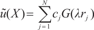$\tilde{u} (X) = \sum_{j = 1}^{N} c_{j} G (λ r_{j})$ (5)

where $N$ is the number of boundary collocation knots, and $c_{j} (j = 1,2, \dots, N)$ are the unknown coefficients, $r = ‖ X - Y ‖$ is the Euclidean norm distance between points $X$ and $Y$ . The non-singular general solutions of Helmholtz equations are written as

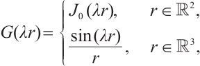$G (λ r) = {\begin{array}{l} J_{0} (λ r), r \in R^{2}, \\ \frac{s i n (λ r)}{r}, r \in R^{3}, \end{array}$ (6)

with $J_{0}$ denoting the Bessel function of the first kind. By collocating the Dirichlet boundary conditions on the boundary collocation knots, i.e., substitute Eq. (5) into Eq. (2), we have

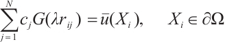$\sum_{j = 1}^{N} c_{j} G (λ r_{i j}) = \bar{u} (X_{i}), X_{i} \in \partial Ω$ (7)

The same procedure can be applied to the Neumann boundary conditions and the Robin boundary conditions. Equation (7) can be directly solved by using the backslash operation in MATLAB.

3 Numerical Experiments

3.1 Case 1

As is known to all, the traditional way to construct numerical solutions is using a function which satisfies the government equation and the corresponding boundary conditions. Here, we consider the exact solution $u = s i n x c o s y$ in a circular domain with radius $r = 1$ with only the Dirichlet boundary conditions. The number of boundary collocation knots is set to $N = 50$ and the number of tested knots is set to $N_{t} = 8 385$ . The node distribution used in our BKM implementation is presented in Fig. 1. Since Cases 2 and 3 employ identical nodal configurations, they are not displayed separately to avoid redundancy.

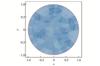Fig. 1 Tested node distribution for Case 1, which is consistently maintained for all test cases

Figure 2 presents the comparative methodological solutions for Case 1, along with the corresponding error distributions interspersed among these approaches. Figure 2(a), (b) and (c) provide the picture of exact solution, BKM numerical solution and partial differential equation (PDE) toolbox solution from MATLAB toolbox, respectively. We can see that the three types of solutions are almost the same. Upon closer inspection, it can be seen that the three different solution types show a striking consistency, indicating a high degree of agreement between their respective results. This result highlights the robustness of the adopted BKM and PDE toolbox methods, as they produce almost indistinguishable results.

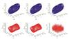Fig. 2 Solutions and error distribution between each two solutions for Case 1

(a) the exact solution $u_{1}$ ; (b) the BKM numerical solution $u_{2}$ ; (c) the PDE toolbox solution $u_{3}$ ; (d) the error distribution $E_{u_{3} - u_{2}}$ between $u_{3}$ and $u_{2}$ against the test points; (e) the error distribution $E_{u_{3} - u_{1}}$ between $u_{3}$ and $u_{1}$ against the test points; (f) the error distribution $E_{u_{2} - u_{1}}$ between $u_{2}$ and $u_{1}$ against the test points.

To see the differences, we consider error distribution between each two solutions against the test points which are shown in Fig. 2(d)-(f), respectively. It should be noted that the average error between the BKM numerical solution and the PDE toolbox solution is 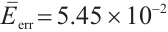${\bar{E}}_{e r r} = 5.45 \times 10^{- 2}$ . The average error between the exact solution and the PDE toolbox solution is also ${\bar{E}}_{e r r} = 5.45 \times 10^{- 2}$ . The average error between the exact solution and the BKM numerical solution is 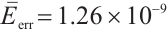${\bar{E}}_{e r r} = 1.26 \times 10^{- 9}$ . This result indicates that the numerical solution obtained from the BKM exhibits greater accuracy in comparison to the solution derived from the PDE toolbox in MATLAB.

3.2 Case 2

Here, the boundary data function is chosen as $u = x^{2} y^{3}$ in a circular domain with only the Dirichlet boundary conditions. We note that there is no exact solution for this case. The boundary collocation number is $N = 50$ and the tested knot number is $N_{t} = 8 385$ .

The BKM numerical solution, the PDE toolbox solution from MATLAB toolbox and the error distribution are shown in Fig.3(a)-(c), respectively. By comparing Fig.3(a) and Fig.3(b), it is evident that the two results are largely consistent with one another. This observation underscores the robustness of both the BKM and the PDE toolbox methods in this particular context, indicating their reliability in producing similar outcomes under the given conditions.

Fig. 3 Solutions and error distribution between the two solutions for Case 2

(a) the BKM numerical solution $u_{2}$ ; (b) the PDE toolbox solution $u_{3}$ ; (c) the error distribution $E_{u_{3} - u_{2}}$ between $u_{3}$ and $u_{2}$ against the test points.

Furthermore, the error distributions between the two solutions against the test points are shown in Fig.3(c), where the average errors between the BKM numerical solution and the PDE solution is ${\bar{E}}_{e r r} = 5.58 \times 10^{- 3}$ . We can see that the result is similar to that of the previous Case 1.

3.3 Case 3

The third case considered boundary data function $u = 1$ on the top semicircle and $u = - 1$ for the rest semicircle in a circular domain with only the Dirichlet boundary conditions. The solution from BKM, PDE toolbox and the error distribution are shown in Fig.4(a)-(c), where the average errors ${\bar{E}}_{e r r} = 2.94$ . We can see that the PDE toolbox solution is very different with the BKM solution.

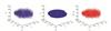Fig. 4 Solutions and error distribution between the two solutions for Case 3

(a) the BKM numerical solution $u_{2}$ ; (b) the PDE toolbox solution $u_{3}$ ; (c) the error distribution $E_{u_{3} - u_{2}}$ between $u_{3}$ and $u_{2}$ against the test points.

Upon comparative analysis of the solutions derived from the PDE toolbox and the BKM method, a significant divergence is observed. This discrepancy suggests that the accuracy of the BKM solution may be compromised in the context of the present case, implying potential limitations in its applicability, the BKM numerical solution may be not accurate for this case.

The limitations of BKM in modeling discontinuous boundaries can be addressed through three principal enhancements: 1) development of hybrid BKM/level-set algorithms^[25-26] for improved interface tracking. 2) implementation of directionally-optimized basis functions for enhanced discontinuity resolution^[27-28]. 3) application of the Tikhonov-type regularization techniques^[17,29] to ensure numerical stability.

4 Conclusion

In this paper, we reassess the efficacy of employing the BKM for solving Helmholtz-type problems by conducting numerical experiments that involve solving equations with various boundary conditions. It is shown that the BKM is effective for problems featuring smooth or continuous boundary conditions. However, it reveals that the BKM may fail when applied to problems with discontinuous boundary conditions. These findings reveal important limitations in the method's current formulation while simultaneously identifying promising research directions. Specifically, future work will focus on two key extensions: (1) adapting the BKM framework to handle fractional derivative problems, and (2) developing improved formulations for discontinuous boundary conditions. These directions represent critical next steps in advancing the method's capabilities and constitute a primary focus of our ongoing research.

References

Pranowo, Wijayanta A T. Numerical solution strategy for natural convection problems in a triangular cavity using a direct meshless local Petrov-Galerkin method combined with an implicit artificial-compressibility model[J]. Engineering Analysis with Boundary Elements, 2021, 126: 13-29. [Google Scholar]
Molaee T, Shahrezaee A. Numerical solution of an inverse source problem for a time-fractional PDE via direct meshless local Petrov-Galerkin method[J]. Engineering Analysis with Boundary Elements, 2022, 138: 211-218. [Google Scholar]
Cui L X, Wu Z M, Xiang H. Quantum radial basis function method for the Poisson equation[J]. Journal of Physics A: Mathematical and Theoretical, 2023, 56(22): 225303. [Google Scholar]
Radmanesh M, Ebadi M J. A local meshless radial basis functions based method for solving fractional integral equations[J]. Computational Algorithms and Numerical Dimensions, 2023, 2(1): 35-46. [Google Scholar]
Lin J, Xu Y T, Reutskiy S, et al. A novel Fourier-based meshless method for (3+1)-dimensional fractional partial differential equation with general time-dependent boundary conditions[J]. Applied Mathematics Letters, 2023, 135: 108441. [Google Scholar]
Ma M L, Xu J, Lu J, et al. The novel backward substitution method for the simulation of three-dimensional time-harmonic elastic wave problems[J]. Applied Mathematics Letters, 2024, 150: 108963. [Google Scholar]
Liu J, Wang F Z, Nadeem S. A new type of radial basis functions for problems governed by partial differential equations[J]. PLoS One, 2023, 18(11): e0294938. [Google Scholar]
Wang F Z, Khan M N, Ahmad I, et al. Numerical solution of traveling waves in chemical kinetics: Time-fractional Fishers equations[J]. Fractals, 2022, 30(2): 2240051. [Google Scholar]
Wang F Z, Shao M Y, Li J L, et al. A space-time domain RBF method for 2D wave equations[J]. Frontiers in Physics, 2023, 11: 1241196. [Google Scholar]
Zhang Z Q, Wang F Z, Zhang J. The space-time meshless methods for the solution of one-dimensional Klein-Gordon equations[J]. Wuhan University Journal of Natural Sciences, 2022, 27(4): 313-320. [Google Scholar]
Kang S W, Lee J M, Kang Y J. Vibration analysis of arbitrarily shaped membranes using non-dimensional dynamic influence function[J]. Journal of Sound and Vibration, 1999, 221(1): 117-132. [Google Scholar]
Ma H W, Wang F Z. New investigations into the BKM for inverse problems of Helmholtz equation[J]. Journal of the Chinese Institute of Engineers, 2016, 39(4): 455-460. [Google Scholar]
Wang F Z, Zheng K H. Analysis of the boundary knot method for 3D Helmholtz-type equation[J]. Mathematical Problems in Engineering, 2014, 2014(1): 853252. [Google Scholar]
Wang F Z, Zheng K H, Li C C, et al. Optimality of the boundary knot method for numerical solutions of 2D Helmholtz-type equations[J]. Wuhan University Journal of Natural Sciences, 2019, 24(4): 314-320. [Google Scholar]
Xuan G X, Zhang W F, Juan Z. Numerical solutions for inverse problems under doubly connected domains[J]. Wuhan University Journal of Natural Science, 2020, 25(4): 323-329. [Google Scholar]
Wang F Z, Ling L, Chen W. Effective condition number for boundary knot method[J]. Computers, Materials & Continua, 2009, 12(1): 57-70. [Google Scholar]
Wang F Z, Chen W, Jiang X R. Investigation of regularized techniques for boundary knot method[J]. International Journal for Numerical Methods in Biomedical Engineering, 2010, 26(12): 1868-1877. [Google Scholar]
Zhang J Y, Wang F Z. Boundary knot method: An overview and some novel approaches[J]. Computer Modeling in Engineering & Sciences, 2012, 88(2): 141-153. [Google Scholar]
Fu Z J, Shi J H, Chen W, et al. Three-dimensional transient heat conduction analysis by boundary knot method[J]. Mathematics and Computers in Simulation, 2019, 165: 306-317. [Google Scholar]
Mužík J. Boundary knot method for convection-diffusion problems[J]. Procedia Engineering, 2015, 111: 582-588. [Google Scholar]
Zhang Q, Ji Z, Sun L L. An improved localized boundary knot method for 3D acoustic problems[J]. Applied Mathematics Letters, 2024, 149: 108900. [Google Scholar]
Lei M, Liu L, Chen C S, et al. The enhanced boundary knot method with fictitious sources for solving Helmholtz-type equations[J]. International Journal of Computer Mathematics, 2023, 100(7): 1500-1511. [Google Scholar]
Jiang X R, Chen W, Chen C S. Fast multipole accelerated boundary knot method for inhomogeneous Helmholtz problems[J]. Engineering Analysis with Boundary Elements, 2013, 37(10): 1239-1243. [Google Scholar]
Shen D J, Lin J, Chen W. Boundary knot method solution of Helmholtz problems with boundary singularities[J]. Journal of Marine Science and Technology, 2014, 22(4): 440-449. [Google Scholar]
Yan F, Feng X T, Lv J H, et al. A continuous-discontinuous hybrid boundary node method for solving stress intensity factor[J]. Engineering Analysis with Boundary Elements, 2017, 81: 35-43. [Google Scholar]
Zhong B D, Yan F, Lv J H. Continuous-discontinuous hybrid boundary node method for frictional contact problems[J]. Engineering Analysis with Boundary Elements, 2018, 87: 19-26. [Google Scholar]
Bernal F, Gutierrez G, Kindelan M. Use of singularity capturing functions in the solution of problems with discontinuous boundary conditions[J]. Engineering Analysis with Boundary Elements, 2009, 33(2): 200-208. [Google Scholar]
Zhang Y M, Sun F L, Young D L, et al. Average source boundary node method for potential problems[J]. Engineering Analysis with Boundary Elements, 2016, 70: 114-125. [Google Scholar]
Qin H H, Wei T, Shi R. Modified Tikhonov regularization method for the Cauchy problem of the Helmholtz equation[J]. Journal of Computational and Applied Mathematics, 2009, 224(1): 39-53. [Google Scholar]

All Figures

	Fig. 1 Tested node distribution for Case 1, which is consistently maintained for all test cases
In the text

Fig. 2 Solutions and error distribution between each two solutions for Case 1

(a) the exact solution $u_{1}$ ; (b) the BKM numerical solution $u_{2}$ ; (c) the PDE toolbox solution $u_{3}$ ; (d) the error distribution $E_{u_{3} - u_{2}}$ between $u_{3}$ and $u_{2}$ against the test points; (e) the error distribution $E_{u_{3} - u_{1}}$ between $u_{3}$ and $u_{1}$ against the test points; (f) the error distribution $E_{u_{2} - u_{1}}$ between $u_{2}$ and $u_{1}$ against the test points.

In the text

	Fig. 3 Solutions and error distribution between the two solutions for Case 2 (a) the BKM numerical solution $u_{2}$ ; (b) the PDE toolbox solution $u_{3}$ ; (c) the error distribution $E_{u_{3} - u_{2}}$ between $u_{3}$ and $u_{2}$ against the test points.
In the text

	Fig. 4 Solutions and error distribution between the two solutions for Case 3 (a) the BKM numerical solution $u_{2}$ ; (b) the PDE toolbox solution $u_{3}$ ; (c) the error distribution $E_{u_{3} - u_{2}}$ between $u_{3}$ and $u_{2}$ against the test points.
In the text

Current usage metrics show cumulative count of Article Views (full-text article views including HTML views, PDF and ePub downloads, according to the available data) and Abstracts Views on Vision4Press platform.

Data correspond to usage on the plateform after 2015. The current usage metrics is available 48-96 hours after online publication and is updated daily on week days.

Initial download of the metrics may take a while.

[1] Pranowo, Wijayanta A T. Numerical solution strategy for natural convection problems in a triangular cavity using a direct meshless local Petrov-Galerkin method combined with an implicit artificial-compressibility model[J]. Engineering Analysis with Boundary Elements, 2021, 126: 13-29. [Google Scholar]

[2] Molaee T, Shahrezaee A. Numerical solution of an inverse source problem for a time-fractional PDE via direct meshless local Petrov-Galerkin method[J]. Engineering Analysis with Boundary Elements, 2022, 138: 211-218. [Google Scholar]

[3] Cui L X, Wu Z M, Xiang H. Quantum radial basis function method for the Poisson equation[J]. Journal of Physics A: Mathematical and Theoretical, 2023, 56(22): 225303. [Google Scholar]

[4] Radmanesh M, Ebadi M J. A local meshless radial basis functions based method for solving fractional integral equations[J]. Computational Algorithms and Numerical Dimensions, 2023, 2(1): 35-46. [Google Scholar]

[5] Lin J, Xu Y T, Reutskiy S, et al. A novel Fourier-based meshless method for (3+1)-dimensional fractional partial differential equation with general time-dependent boundary conditions[J]. Applied Mathematics Letters, 2023, 135: 108441. [Google Scholar]

[6] Ma M L, Xu J, Lu J, et al. The novel backward substitution method for the simulation of three-dimensional time-harmonic elastic wave problems[J]. Applied Mathematics Letters, 2024, 150: 108963. [Google Scholar]

[7] Liu J, Wang F Z, Nadeem S. A new type of radial basis functions for problems governed by partial differential equations[J]. PLoS One, 2023, 18(11): e0294938. [Google Scholar]

[8] Wang F Z, Khan M N, Ahmad I, et al. Numerical solution of traveling waves in chemical kinetics: Time-fractional Fishers equations[J]. Fractals, 2022, 30(2): 2240051. [Google Scholar]

[9] Wang F Z, Shao M Y, Li J L, et al. A space-time domain RBF method for 2D wave equations[J]. Frontiers in Physics, 2023, 11: 1241196. [Google Scholar]

[10] Zhang Z Q, Wang F Z, Zhang J. The space-time meshless methods for the solution of one-dimensional Klein-Gordon equations[J]. Wuhan University Journal of Natural Sciences, 2022, 27(4): 313-320. [Google Scholar]

[11] Kang S W, Lee J M, Kang Y J. Vibration analysis of arbitrarily shaped membranes using non-dimensional dynamic influence function[J]. Journal of Sound and Vibration, 1999, 221(1): 117-132. [Google Scholar]

[12] Ma H W, Wang F Z. New investigations into the BKM for inverse problems of Helmholtz equation[J]. Journal of the Chinese Institute of Engineers, 2016, 39(4): 455-460. [Google Scholar]

[13] Wang F Z, Zheng K H. Analysis of the boundary knot method for 3D Helmholtz-type equation[J]. Mathematical Problems in Engineering, 2014, 2014(1): 853252. [Google Scholar]

[14] Wang F Z, Zheng K H, Li C C, et al. Optimality of the boundary knot method for numerical solutions of 2D Helmholtz-type equations[J]. Wuhan University Journal of Natural Sciences, 2019, 24(4): 314-320. [Google Scholar]

[15] Xuan G X, Zhang W F, Juan Z. Numerical solutions for inverse problems under doubly connected domains[J]. Wuhan University Journal of Natural Science, 2020, 25(4): 323-329. [Google Scholar]

[16] Wang F Z, Ling L, Chen W. Effective condition number for boundary knot method[J]. Computers, Materials & Continua, 2009, 12(1): 57-70. [Google Scholar]

[17] Wang F Z, Chen W, Jiang X R. Investigation of regularized techniques for boundary knot method[J]. International Journal for Numerical Methods in Biomedical Engineering, 2010, 26(12): 1868-1877. [Google Scholar]

[18] Zhang J Y, Wang F Z. Boundary knot method: An overview and some novel approaches[J]. Computer Modeling in Engineering & Sciences, 2012, 88(2): 141-153. [Google Scholar]

[19] Fu Z J, Shi J H, Chen W, et al. Three-dimensional transient heat conduction analysis by boundary knot method[J]. Mathematics and Computers in Simulation, 2019, 165: 306-317. [Google Scholar]

[20] Mužík J. Boundary knot method for convection-diffusion problems[J]. Procedia Engineering, 2015, 111: 582-588. [Google Scholar]

[21] Zhang Q, Ji Z, Sun L L. An improved localized boundary knot method for 3D acoustic problems[J]. Applied Mathematics Letters, 2024, 149: 108900. [Google Scholar]

[22] Lei M, Liu L, Chen C S, et al. The enhanced boundary knot method with fictitious sources for solving Helmholtz-type equations[J]. International Journal of Computer Mathematics, 2023, 100(7): 1500-1511. [Google Scholar]

[23] Jiang X R, Chen W, Chen C S. Fast multipole accelerated boundary knot method for inhomogeneous Helmholtz problems[J]. Engineering Analysis with Boundary Elements, 2013, 37(10): 1239-1243. [Google Scholar]

[24] Shen D J, Lin J, Chen W. Boundary knot method solution of Helmholtz problems with boundary singularities[J]. Journal of Marine Science and Technology, 2014, 22(4): 440-449. [Google Scholar]

[25] Yan F, Feng X T, Lv J H, et al. A continuous-discontinuous hybrid boundary node method for solving stress intensity factor[J]. Engineering Analysis with Boundary Elements, 2017, 81: 35-43. [Google Scholar]

[26] Zhong B D, Yan F, Lv J H. Continuous-discontinuous hybrid boundary node method for frictional contact problems[J]. Engineering Analysis with Boundary Elements, 2018, 87: 19-26. [Google Scholar]

[27] Bernal F, Gutierrez G, Kindelan M. Use of singularity capturing functions in the solution of problems with discontinuous boundary conditions[J]. Engineering Analysis with Boundary Elements, 2009, 33(2): 200-208. [Google Scholar]

[28] Zhang Y M, Sun F L, Young D L, et al. Average source boundary node method for potential problems[J]. Engineering Analysis with Boundary Elements, 2016, 70: 114-125. [Google Scholar]

[29] Qin H H, Wei T, Shi R. Modified Tikhonov regularization method for the Cauchy problem of the Helmholtz equation[J]. Journal of Computational and Applied Mathematics, 2009, 224(1): 39-53. [Google Scholar]