| Issue |
Wuhan Univ. J. Nat. Sci.
Volume 30, Number 4, August 2025
|
|
|---|---|---|
| Page(s) | 313 - 320 | |
| DOI | https://doi.org/10.1051/wujns/2025304313 | |
| Published online | 12 September 2025 | |
CLC number: TP242.2
Fault Detection of Industrial Robot Drive Systems: An Enhanced Unscented Kalman Filter Approach
工业机器人驱动系统故障检测:一种增强型UKF方法
1
School of Internet of Things Engineering, Wuxi Taihu University, Wuxi 214000, Jiangsu, China
2
Provincial Key (Construction) Laboratory of Intelligent Internet of Things Technology and Applications in Universities, Wuxi 214000, Jiangsu, China
3
School of Computer Science and Artificial Intelligence, Changzhou University, Changzhou 213000, Jiangsu, China
Received:
18
December
2024
Abstract
Fault detection in industrial robot drive systems is a critical aspect of ensuring operational reliability and efficiency. To address the challenge of balancing accuracy and robustness in existing fault detection methods, this paper proposes an enhanced fault detection method based on the unscented Kalman filter (UKF). A comprehensive mathematical model of the brushless DC motor drive system is developed to provide a theoretical foundation for the design of subsequent fault detection methods. The conventional UKF estimation process is detailed, and its limitations in balancing estimation accuracy and robustness are addressed by introducing a dynamic, time-varying boundary layer. To further enhance detection performance, the method incorporates residual analysis using improved z-score and signal-to-noise ratio (SNR) metrics. Numerical simulations under both fault-free and faulty conditions demonstrate that the proposed approach achieves lower root mean square error (RMSE) in fault-free scenarios and provides reliable fault detection. These results highlight the potential of the proposed method to enhance the reliability and robustness of fault detection in industrial robot drive systems.
摘要
工业机器人驱动系统故障检测是确保其可靠高效运行的关键。针对现有故障检测方法中精度与鲁棒性难以平衡的问题,本文提出一种基于无迹卡尔曼滤波器(UKF)的增强型故障检测方法。通过建立无刷直流电机驱动系统的完整数学模型,为后续的故障检测方法设计提供理论支持。在阐述传统UKF的估计过程基础上,通过引入动态时变边界层来解决其估计精度与鲁棒性难以平衡的局限。所提方法融合了改进z-score和信噪比(SNR)的残差分析方法,以进一步提升故障检测性能。在无故障和故障工况下的数值仿真表明,该方法在无故障工况下具有更低均方根误差(RMSE),且能实现可靠故障检测。研究结果验证了此方法在提升工业机器人驱动系统故障检测可靠性和鲁棒性方面的潜力。
Key words: fault detection / industrial robot / enhanced unscented Kalman filter (UKF)
关键字 : 故障检测 / 工业机器人 / 增强型UKF
Cite this article: LIU Chen, ZHU Chenyang. Fault Detection of Industrial Robot Drive Systems: An Enhanced Unscented Kalman Filter Approach[J]. Wuhan Univ J of Nat Sci, 2025, 30(4): 313-320.
Biography: LIU Chen, female, Lecturer, research direction: fault detection and diagnosis. E-mail: This email address is being protected from spambots. You need JavaScript enabled to view it.
Foundation item: Supported by the Natural Science Foundation of the Higher Education Institutions of Jiangsu Province (22KJB520012), the Research Project on Higher Education Reform in Jiangsu Province (2023JSJG781) and the College Student Innovation and Entrepreneurship Training Program Project (202313571008Z)
© Wuhan University 2025
 This is an Open Access article distributed under the terms of the Creative Commons Attribution License (https://creativecommons.org/licenses/by/4.0), which permits unrestricted use, distribution, and reproduction in any medium, provided the original work is properly cited.
0 Introduction
Industrial robots are integral to modern automation technologies, extensively utilized in manufacturing for tasks such as assembly, welding, material handling, and precision machining. The drive system, as the core of an industrial robot, ensures precise movement and operational efficiency. However, these systems are susceptible to faults in their drive control mechanisms, which can degrade performance, reduce productivity, or even lead to catastrophic failures[1-2]. As the adoption of industrial robots grows, fault detection and diagnosis in drive systems have become critical for ensuring reliability and minimizing operational downtime[3].
One of the earliest approaches to improving system reliability, hardware redundancy, involves duplicating critical components to maintain operation during faults[4-5]. Although effective, this approach increases system cost, weight, and complexity, making it less desirable for modern applications. In contrast, model-based analytical methods leverage mathematical models to represent nominal system behavior and detect anomalies by comparing predicted outputs with actual observations[6]. These methods offer distinct advantages over hardware redundancy by enabling the detection of subtle faults and providing deeper insights into system dynamics. Among model-based methods, the Kalman filter (KF), a recursive algorithm, is widely employed to estimate the state of dynamic systems from noisy measurements. The KF has been extensively studied and applied across various fields[7]. For instance, Lee et al[8] developed a fault detection and diagnosis (FDD) algorithm for an open-cycle liquid propellant rocket engine using a conventional KF. Similarly, a residual generator based on the KF was proposed in Ref. [9] to diagnose faults and achieve fault-tolerant control in linear drive systems. However, despite its success, the KF's application is limited in systems exhibiting nonlinear dynamics, which are prevalent in physical and industrial systems.
To address the challenges posed by nonlinearity, advanced variants of the KF, such as the extended Kalman filter (EKF), unscented Kalman filter (UKF), and particle filter (PF), have been developed. The EKF, which linearizes nonlinear systems via Taylor series expansion, has been employed in various applications. For instance, Gao et al[10] proposed an EKF-based fault diagnosis strategy for unmanned aerial vehicles, integrating multiple-model adaptive estimation to diagnose actuator faults efficiently. Similarly, an EKF-based fault detection model for the papermaking wastewater treatment process was introduced in Ref. [11]. However, the EKF's reliance on linearization introduces approximation errors, motivating the development of the UKF, which uses sigma-point sampling to achieve more accurate approximations of nonlinear dynamics. For example, Tian et al[12] proposed a UKF-based online estimation algorithm for insulation resistance in battery energy storage systems. Furthermore, a distributed UKF framework for sensor fault detection, isolation, and accommodation was presented in Ref. [13]. While the particle filter offers another alternative by using particle sampling, its effectiveness can be compromised by state estimation inaccuracies[14]. To mitigate this, Yin et al[15] enhanced the PF with genetic algorithms to detect faults in a three-tank system. Despite these advancements, traditional KF-based FDD methods often neglect robustness and stability in state estimation, particularly in handling model uncertainties, external disturbances, and noise.
Industrial robot drive systems operate in complex environments subject to such disturbances, necessitating more robust fault detection frameworks. In this paper, we propose an enhanced UKF-based fault detection method to address these challenges. A dynamic time-varying boundary layer is incorporated into the UKF framework to balance estimation accuracy and robustness. Robust state estimates are used to generate residuals by comparing them with actual system outputs. To further improve fault detection reliability, z-score analysis, and signal-to-noise ratio (SNR) analysis are integrated into the detection process. This combined approach ensures efficient and accurate fault detection in industrial robot drive systems.
The remaining sections are structured as follows: Section 1 reviews the mathematical formulation of the drive system and the convention UKF algorithm. In Section 2, an enhanced UKF algorithm is introduced. Subsequently, Section 3 proposes the fault detection scheme. Section 4 presents the numerical simulation cases for validating the proposed method. The conclusion is drawn in Section 5.
1 Preliminary
This section presents the mathematical model of the industrial robot drive system to accurately describe its dynamic characteristics and illustrates the algorithm for state estimation using the traditional UKF.
1.1 Modeling of the Drive System
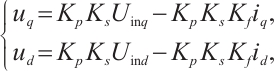
The joints of industrial robot arms require motor drives with high precision, high reliability, and high torque characteristics. The brushless DC motor, which meets these requirements, is widely used in industrial robots. A typical brushless DC motor drive system includes the motor body, sinusoidal pulse width modulation (SPWM) inverter, and current feedback loop, as shown in the structure of Fig. 1. Based on the effect of current feedback, the relationships between the system's current, voltage, and control vector, after applying the Park transformation, can be expressed as follows:
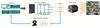 |
Fig. 1 Schematic diagram of brushless DC motor drive systems |
 (1)
(1)
where  and
and  are the voltages applied to the
  -axis and
  -axis, respectively.
  and
and  are the currents flowing through the
  -axis and
  -axis.
  ,
,  , and
, and  represent the current controller gain, the equivalent gain of the inverter, and the current feedback parameter.
  and
and  are the reference signals for the
  -axis and
  -axis, respectively.
To achieve a higher torque coefficient and a bidirectional symmetric linear current-torque characteristic, the rotor position sensor is typically installed such that the reference phasor aligns with the  -axis, i.e.,
  , and
, and  is numerically equal to the control input
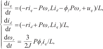
  . Additionally, for a motor body, its state can be expressed as follows.
 (2)
(2)
where  and
and  are the winding resistance and self-induction coefficient.
  is the rotor inertia.
  stands for the number of poles.
  is the flux linkage generated by permanent magnetic poles and the stator winding. While
  indicates the motor speed.
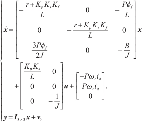
Considering the accuracy requirements of the mathematical model, the effect of the no-load torque should not be neglected. Combining the previous descriptions with equations (1) and (2), the final mathematical model of the brushless DC motor in the  -
- coordinate frame is expressed as follows:
 (3)
(3)
where 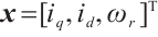 is defined as the state vector.
 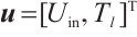 represents the control vector consisting of the input reference voltage and load torque.
  is the rotor damping coefficient.
  is the identity matrix.
  denotes the measurement noise. Clearly, equation (3) presents a fully measurable nonlinear system. In the UKF, the unscented transform can effectively approximate the characteristics of the target system.
1.2 Estimation with the Conventional UKF
By using sigma points to propagate the state distribution through nonlinear transformations, the conventional UKF can handle complex nonlinearities without the need for linearization, making it particularly suitable for applications in industry robotics, where accurate state estimation is critical. The UKF consists of three main phases: sigma point generation, prediction step, and update step, which is iteratively applied to estimate the state and its covariance.
a) Sigma point generation
At each time step, the UKF begins by generating a set of sigma points  based on the current state estimate
  and the associated covariance matrix
  .
.
 (4)
(4)
where  is the dimension of
  .
.  denotes the state covariance matrix.
  is a scaling parameter that controls the spread of the sigma points around the mean state estimate.
b) Prediction step
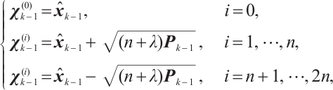
In the prediction phase, the  sigma points are propagated through the nonlinear process model, as presented in equation (3). For ease of reading, the target system (3) is represented in a compact form
  . Thus, one has
 (5)
(5)
where  denotes the predicted sigma points at time
  . Subsequently, the predicted state estimate and covariance can be obtained as the weighted average of the sigma points, as shown in equation (6).
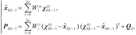 (6)
(6)
where  and
and  are the weights for the mean and covariance, respectively.
  denotes the process noise covariance.
c) Update step
In the update phase, the predicted sigma points are passed through the nonlinear measurement model (not including the measurement noise), denoted as  , resulting in the measurement and prediction similarly:
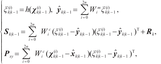 (7)
(7)
where  denotes the measurement noise covariance.
  denotes the predicted measurement covariance.
  is the cross-covariance matrix. Based on (7), the innovation gain
  is readily calculated as:
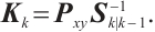 (8)
(8)
Finally, the state estimate  and its covariance
  are updated as follows:
 (9)
(9)
where  denotes the actual measurement at time
  .
.
2 Enhanced UKF for Robust Estimation
As seen from equations (8) and (9) in the UKF algorithm, the state estimation is achieved by using the innovation gain  . This approach typically yields high estimation accuracy. Nonetheless, ensuring reliable state estimation despite system uncertainties or external noise continues to be a significant challenge.
In addressing the trade-off between accurate estimation and robustness against disturbances, we are inspired by the variable structure filters presented in Refs. [16-17]. We incorporate a sliding boundary layer into the UKF gain update process to enhance the robustness of the estimation. The enhanced innovation gain is defined as follows:
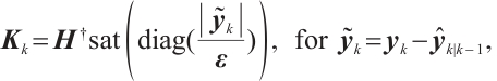 (10)
(10)
where  is the sliding boundary layer to be designed.
  denotes the pseudoinverse of the measurement matrix
  .
.  ,
,  , and
, and  represent the absolute, saturation, and diagonal operations, respectively. By replacing the conventional innovation gain
  in (8) with the enhanced one in (10), the state estimation in the UKF is forced to converge within a boundary layer
  .
.
Clearly, the selection of the boundary layer width is crucial. The simplest approach is to set a fixed width based on the system's maximum uncertainty. However, this method lacks flexibility. Therefore, we next focus on designing an adaptive time-varying boundary layer to adapt to the dynamic estimation process.
Based on (10), and utilizing a first-order Taylor approximation, one has the posterior error as follows:
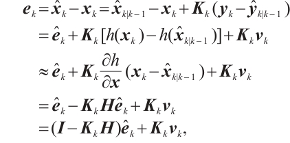 (11)
(11)
where 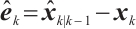 denotes the prior error.
  is the Jacobian matrix with respect to
  . Consequently, the state error covariance matrix
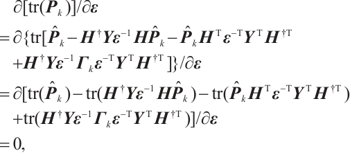
  is readily calculated as (12), which indicates the characteristics of the estimated state.
 (12)
(12)
 is the prior state error covariance.
  represents the measurement noise covariance as described before. It is evident that
  is a function of the boundary layer parameter
  , and thus, the optimal value of
  can be determined by minimizing the trace of
  , i.e.,
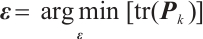 (13)
(13)
For ease of calculation, the enhanced innovation gain in (10) is denoted in a compact form 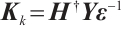 , where
  and
and  represent the saturation of associated diagonal elements in (10), respectively. Therefore, by combining (12), the optimal solution to (13) is calculated as follows:
 (14)
(14)
where 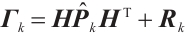 . By applying the matrix trace operation rules to the terms in (14), the equation is simplified as:
 (15)
(15)
For (15), the solution can be easily obtained as:
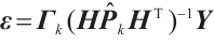 (16)
(16)
Combining equations (9), (10), and (16), one obtains the new state estimation with the enhanced innovation gain, as expressed in equation (17).
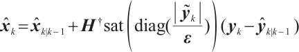 (17)
(17)
Obviously, by introducing a switching term in the state estimation, the estimated state is driven to converge within the boundary layer. Unlike traditional smooth variable structure filters (SVSF, refer to Refs. [16-17]), the time-varying boundary layer proposed in this paper employs a saturation function, denoted as  , instead of a sign function, denoted as
  , which mitigates the chattering phenomenon, as illustrated in Fig. 2. Note that
  incorporates both the state covariance and measurement error (see equation (16)), which presents the system uncertainties and measurement noise during the estimation process. This is precisely why the proposed method enhances the robustness of the estimation.
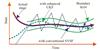 |
Fig. 2 State estimation comparison with different methods |
3 Fault Detection Strategy
As mentioned earlier, fault detection is crucial when anomalies occur in the industrial robot drive system. The generation and analysis of residuals serve as the fundamental basis for fault detection. This section will focus on the fault detection framework and residual analysis methods based on the enhanced UKF.
3.1 Fault Detection Framework
The fault detection process based on the enhanced UKF is initiated by estimating the system state using the enhanced UKF algorithm detailed in Section 2. This state estimation provides a reference for subsequent analysis. Subsequently, residuals are generated by comparing the actual system outputs with the estimates from the enhanced UKF model. These residuals encapsulate the discrepancies between the actual and expected behaviors of the system, serving as primary indicators of potential faults. The principle framework for fault detection is shown in Fig. 3.
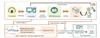 |
Fig. 3 Principle fault detection framework based on the enhanced UKF |
Specifically, to ensure the reliability and effectiveness of the fault detection framework, a comprehensive monitoring system is established. As shown in Fig. 3, the fault detection system tracks performance metrics of the industrial robot drive system, such as motor speed  and current fluctuations of
  and
and  , as illustrated in equation (3). By integrating these monitored data with the residual analysis, a more holistic understanding of the system's health status is achieved.
3.2 Residual Analysis
This paper first applies the improved z-score method for normalization. The z-score process is given by the following formula:
 (18)
(18)
where  represents the median operation.
  is the residual vector at time
  (shown as "residual" in Fig.3). Additionally,
  represents a residual set consisting of a window of residual samples with the length of
  . Without using the insensitive mean and standard deviation in the traditional z-score, the improved z-score is based on the median and median absolute deviation, providing a better measure of central tendency and dispersion for skewed or non-normal data[18]. Therefore, the improved z-score offers an effective way of indicating potential anomalies in the residual signals.
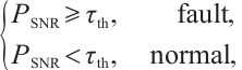
Considering the measurement noise or unknown external disturbances affecting the residuals, misleading results of the improved z-score, we treat the normalized results  as noise-contaminated signals and apply the SNR method for filtering to detect anomalies, calculated as follows.
 (19)
(19)
where  and
and  represent the mean operation and variance operation, respectively.
  is a set of
  within a window of
  samples.
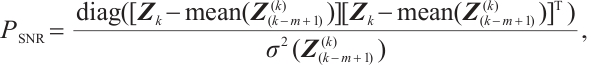
The SNR metric in equation (19) can be understood as the ratio of the power of specific correlated noise to the average power of the entire sampling noise. When the system is operating normally, the SNR metric has a lower value. However, when a fault occurs, the PSNR metric will display higher amplitudes, as illustrated in the following rule:
 (20)
(20)
where  represents the threshold, selected as the mean of
  over a window of samples from the initial fault-free moment.
4 Numeral Simulation
This section validates the effectiveness of the proposed method (denoted as EUKF) through two simulation cases and compares it with the traditional UKF method in Ref. [19] (denoted as UKF) and the adaptive robust UKF method proposed in Ref. [20] (denoted as ARUKF). To initiate the simulation, the parameters of the brushless DC motor are configured as follows.  ,
,  ,
,  ,
,  ,
,  ,
,  , and
, and  . The measurement noise is Gaussian white noise with a power level of
  . Moreover, the sampling step is configured as
  .
.
4.1 Case 1: Robust Estimation Performance under Fault-Free Conditions
To validate the robustness of the proposed method, in this case, the system is subjected to Gaussian white noise interference without any faults occurring, and the initial value of the system state is set to  . To save space, we only plot the
  state output and the estimation curves of different methods in the left subplot of Fig. 4, where the actual output is labelled as
  , and state estimates of the different methods are labelled with EUKF, ARUKF, and UKF. To clearly illustrate the estimation errors of different methods under noise interference, we present the estimation error curves (as labelled with Err) and box plots for the different methods on the right of Fig. 4. Furthermore, for ease of comparison, RMSE statistics of different estimation errors are provided in Table 1. The statistics show that, for all state estimations, the proposed method EUKF exhibits the smallest RMSE compared to the other methods, demonstrating the robustness of the proposed enhanced UKF.
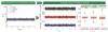 |
Fig. 4 State estimations and estimation errors with different methods for 
|
RMSE statistics for state estimation errors under different methods
4.2 Case 2: Fault Detection under Fault Conditions
Due to the complex working environment and continuous long-term operation of industrial robots, the drive system is prone to failures, such as increased operating temperature and lubrication failure, which can lead to sudden abnormalities in the motor rotor damping parameter  . In this case, it is assumed that
  changes from
  to
to  between 2.6 s and 2.63 s. Residuals are generated using the proposed method to perform fault detection. Similarly, the state estimation and fault detection results for
  are illustrated in Fig. 5.
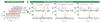 |
Fig. 5 State estimation and fault detection for  under the fault condition under the fault condition
|
From the state estimation results in Fig. 5 (shown in the left subplot), it can be observed that when  experiences an anomaly, the system state
  deviates from its normal value, and the estimation results of all methods exhibit fluctuations. The SNR results for each comparative method are shown in the three subplots on the right,
labelled as PSNR-EUKF, PSNR-ARUKF, and PSNR-UKF. The corresponding thresholds are labelled as τ-EUKF, τ-ARUKF, and τ-UKF. When an anomaly occurs, the SNR statistics can quickly detect the system anomaly and exceed the anomaly threshold. To visually compare the fault detection results of different methods, we statistically analyze the false detection rate (FDR) and missed detection rate (MDR) for each state (i.e.,  ,
,  , and
, and  ) with different methods, as shown in Table 2. The data show that EUKF, compared with the other methods, achieves the lowest FDR and MDR across all states. This indicates that the proposed state estimation and residual analysis strategy provides the best performance for fault detection in the system.
FDR and MDR for each state with different methods %
5 Conclusion
This paper presents an enhanced unscented Kalman filter (EUKF) approach for fault detection in industrial robot drive systems. By incorporating a dynamic, time-varying boundary layer into the UKF and using a combination of improved z-score and SNR analysis for residual evaluation, the proposed method achieves a better trade-off between estimation accuracy and robustness. The numerical simulation results under fault-free and faulty conditions suggest that the proposed approach can enhance the reliability and efficiency of fault detection in industrial robot drive systems.
Future work will focus on extending the proposed method to handle more complex fault scenarios and integrating it with fault-tolerant control strategies to improve the overall performance and safety of industrial robots.
References
- Kim Y, Park J, Na K, et al. Phase-based time domain averaging (PTDA) for fault detection of a gearbox in an industrial robot using vibration signals[J]. Mechanical Systems and Signal Processing, 2020, 138: 106544. [Google Scholar]
- Vallachira S, Orkisz M, Norrlöf M, et al. Data-driven gearbox failure detection in industrial robots[J]. IEEE Transactions on Industrial Informatics, 2020, 16(1): 193-201. [Google Scholar]
- Gillini G, Lippi M, Arrichiello F, et al. Distributed fault detection and isolation for cooperative mobile manipulators[C]//2019 IEEE International Conference on Systems, Man and Cybernetics (SMC). New York: IEEE, 2019: 1701-1707. [Google Scholar]
- Barbirotta M, Menichelli F, Cheikh A, et al. Dynamic triple modular redundancy in interleaved hardware threads: An alternative solution to lockstep multi-cores for fault-tolerant systems[J]. IEEE Access, 2024, 12: 95720-95735. [Google Scholar]
- Mehdi S, Mehdi A. New hardware redundancy approach for making modules tolerate faults using a new fault detecting voter unit structure[J]. IET Circuits, Devices & Systems, 2020, 14(7): 980-989. [Google Scholar]
- Abid A, Khan M T, Iqbal J. A review on fault detection and diagnosis techniques: Basics and beyond[J]. Artificial Intelligence Review, 2021, 54(5): 3639-3664. [Google Scholar]
- Afshari H H, Gadsden S A, Habibi S. Gaussian filters for parameter and state estimation: A general review of theory and recent trends[J]. Signal Processing, 2017, 135: 218-238. [Google Scholar]
- Lee K, Cha J, Ko S, et al. Fault detection and diagnosis algorithms for an open-cycle liquid propellant rocket engine using the Kalman filter and fault factor methods[J]. Acta Astronautica, 2018, 150: 15-27. [Google Scholar]
- Huang S N, Tan K K, Lee T H. Fault diagnosis and fault-tolerant control in linear drives using the Kalman filter[J]. IEEE Transactions on Industrial Electronics, 2012, 59(11): 4285-4292. [Google Scholar]
- Gao J X, Zhang Q, Chen J Y. EKF-based actuator fault detection and diagnosis method for tilt-rotor unmanned aerial vehicles[J]. Mathematical Problems in Engineering, 2020, 2020(1): 8019017. [Google Scholar]
- Niu G Q, Liu Y, Zhou J, et al. SBR-extended Kalman filter model-based fault diagnosis and signal reconstruction for the papermaking wastewater treatment process[J]. Journal of Water Process Engineering, 2023, 56: 104420. [Google Scholar]
- Tian J Q, Liu X H, Zhang Q P, et al. Insulation fault diagnosis of battery pack based on adaptive filtering algorithm[J]. IEEE Transactions on Dielectrics and Electrical Insulation, 2024, 31(1): 495-504. [Google Scholar]
- Shaheen K, Chawla A, Uilhoorn F E, et al. Sensor-fault detection, isolation and accommodation for natural-gas pipelines under transient flow[J]. IEEE Transactions on Signal and Information Processing over Networks, 2024, 10: 264-276. [Google Scholar]
- Shao S, Bi J, Yang F, et al. Online estimation of state-of-charge of Li-ion batteries in electric vehicle using the resampling particle filter[J]. Transportation Research Part D: Transport and Environment, 2014, 32: 207-217. [Google Scholar]
- Yin S, Zhu X P. Intelligent particle filter and its application to fault detection of nonlinear system[J]. IEEE Transactions on Industrial Electronics, 2015, 62(6): 3852-3861. [Google Scholar]
- Avzayesh M, Abdel-Hafez M, AlShabi M, et al. The smooth variable structure filter: A comprehensive review[J]. Digital Signal Processing, 2021, 110: 102912. [Google Scholar]
- Wang L, Ma J, Zhao X, et al. Online estimation of state-of-charge inconsistency for lithium-ion battery based on SVSF-VBL[J]. Journal of Energy Storage, 2023, 67: 107657. [Google Scholar]
- Madjidi H, Laroussi T, Farah F. A robust and fast CFAR ship detector based on Median absolute deviation thresholding for SAR imagery in heterogeneous log-normal sea clutter[J]. Signal, Image and Video Processing, 2023, 17(6): 2925-2931. [Google Scholar]
- Xiong K, Chan C W, Zhang H Y. Unscented Kalman filter for fault detection[J]. IFAC Proceedings Volumes, 2005, 38(1): 113-118. [Google Scholar]
- Ding H C, Qin X J, Wei L C. Sensorless control of surface-mounted permanent magnet synchronous motor using adaptive robust UKF[J]. Journal of Electrical Engineering & Technology, 2022, 17(5): 2995-3013. [Google Scholar]
All Tables
All Figures
|
Fig. 1 Schematic diagram of brushless DC motor drive systems |
| In the text | |
|
Fig. 2 State estimation comparison with different methods |
| In the text | |
|
Fig. 3 Principle fault detection framework based on the enhanced UKF |
| In the text | |
|
Fig. 4 State estimations and estimation errors with different methods for
|
| In the text | |
|
Fig. 5 State estimation and fault detection for under the fault condition
|
| In the text | |
Current usage metrics show cumulative count of Article Views (full-text article views including HTML views, PDF and ePub downloads, according to the available data) and Abstracts Views on Vision4Press platform.
Data correspond to usage on the plateform after 2015. The current usage metrics is available 48-96 hours after online publication and is updated daily on week days.
Initial download of the metrics may take a while.