| Issue |
Wuhan Univ. J. Nat. Sci.
Volume 30, Number 4, August 2025
|
|
|---|---|---|
| Page(s) | 321 - 333 | |
| DOI | https://doi.org/10.1051/wujns/2025304321 | |
| Published online | 12 September 2025 | |
CLC number: TP212
Distributed Fiber Optic Vibration Sensing Event Recognition Method Based on CNN-LSTM-Transformer Net
基于CNN-LSTM-Transformer网格的分布式光纤振动传感事件识别方法
1
College of Optoelectronic Information and Computer Engineering, University of Shanghai for Science and Technology, Shanghai 200093, China
2
School of Electronic and Electrical Engineering, Shanghai University of Engineering Science, Shanghai 201620, China
3
Key Laboratory of Space Active Optical-Electro Technology, Chinese Academy of Sciences, Shanghai 200083, China
Received:
24
January
2025
Abstract
Phase-sensitive Optical Time-Domain Reflectometer ( -OTDR) technology facilitates the real-time detection of vibration events along fiber optic cables by analyzing changes in Rayleigh scattering signals. This technology is widely used in applications such as intrusion monitoring and structural health assessments. Traditional signal processing methods, such as Support Vector Machines (SVM) and K-Nearest Neighbors (KNN), have limitations in feature extraction and classification in complex environments. Conversely, a single deep learning model often struggles with capturing long time-series dependencies and mitigating noise interference. In this study, we propose a deep learning model that integrates Convolutional Neural Network (CNN), Long Short-Term Memory Network (LSTM), and Transformer modules, leveraging
  -OTDR technology for distributed fiber vibration sensing event recognition. The hybrid model combines the CNN's capability to extract local features, the LSTM's ability to model temporal dynamics, and the Transformer's proficiency in capturing global dependencies. This integration significantly enhances the accuracy and robustness of event recognition. In experiments involving six types of vibration events, the model consistently achieved a validation accuracy of 0.92, and maintained a validation loss of approximately 0.2, surpassing other models, such as TAM+BiLSTM and CNN+CBAM. The results indicate that the CNN+LSTM+Transformer model is highly effective in handling vibration signal classification tasks in complex scenarios, offering a promising new direction for the application of fiber optic vibration sensing technology.
摘要
相位敏感光时域反射计( -OTDR)技术通过分析瑞利散射信号的变化,实现对光缆沿线振动事件的实时检测,广泛应用于入侵监测、结构健康评估等领域。传统的信号处理方法(如 SVM、KNN 等)在特征提取及复杂场景分类上存在局限,而单一深度学习模型在长时序依赖捕捉及噪声干扰方面效果不佳。本文基于
  -OTDR技术,提出了一种融合 CNN、LSTM 和 Transformer 模块的深度学习模型,用于分布式光纤振动传感事件的识别。提出的混合模型结合 CNN 提取局部特征、LSTM 建模时序动态、Transformer 捕获全局依赖关系,显著提升了识别的精度和鲁棒性。在对 6 类振动事件的实验中,该模型验证准确率稳定在0.92,验证损失在 0.2左右,优于其他对比模型(如 TAM+BiLSTM 和 CNN+CBAM)。研究表明,CNN+LSTM+Transformer 通过其全局建模与特征融合优势,能够有效应对复杂场景下的振动信号分类任务,为光纤振动传感技术的应用提供了新的方向。
Key words: distributed fiber optic vibration sensing / convolutional neural network / long and short-term memory network / attention mechanism / φ-OTDR
关键字 : 分布式光纤振动传感 / 卷积神经网络 / 长短期记忆网络 / 注意力机制 / φ-OTDR
Cite this article: LI Jun, WANG Liqun, LIU Jin, et al. Distributed Fiber Optic Vibration Sensing Event Recognition Method Based on CNN-LSTM-Transformer Net[J]. Wuhan Univ J of Nat Sci, 2025, 30(4):321-333.
Biography: LI Jun, female, Ph.D., Associate professor, research direction: signal analysis and processing, automation control and digital image processing, etc. E-mail: This email address is being protected from spambots. You need JavaScript enabled to view it.
Foundation item: Supported by Key Laboratory of Space Active Optical-Electro Technology of Chinese Academy of Sciences (2021ZDKF4)
© Wuhan University 2025
 This is an Open Access article distributed under the terms of the Creative Commons Attribution License (https://creativecommons.org/licenses/by/4.0), which permits unrestricted use, distribution, and reproduction in any medium, provided the original work is properly cited.
0 Introduction
Phase-sensitive optical time-domain reflectometer ( -OTDR), as a new fiber-optic sensing technology[1], utilizes the Rayleigh scattering phenomenon in optical fibers for real-time detection of vibration and strain. This technique involves transmitting a pulsed light signal through an optical fiber, which interacts with minor inhomogeneities (such as vibrations and temperature variations) within the fiber. These interactions result in variations in the Rayleigh scattering signal. By analyzing the phase changes of these echo signals, vibration events and their corresponding locations along the fiber can be precisely detected.
  -OTDR offers significant advantages over traditional fiber-optic sensing technologies such as fiber Bragg gratings (FBG) and interferometric fiber optic sensors (FPI). While conventional techniques tend to provide only a limited number of sensing points,
  -OTDR is capable of continuous real-time monitoring along the entire length of the fiber, providing vibration information at each monitoring point. Its high spatial resolution makes it possible to pinpoint even the smallest vibration events in the fiber and maintain highly accurate monitoring over long distances (tens of kilometers)[2]. The development of
  -OTDR technology is of great significance for the effective real-time monitoring of single-mode fiber vibrations, as it can efficiently monitor perimeter intrusion signals, pipeline safety, seismic detection, underwater cable monitoring, structural health detection, and other fields[3-4].
A distributed fiber optic vibration sensing (DVS) system is based on  -OTDR technology. The basic principle is to inject light pulses into the sensing fiber optic cable and obtain the environmental state changes along the fiber optic cable by receiving and analyzing the Rayleigh signals backscattered in the fiber optic cable. Because optical fibers are extremely sensitive to external vibration, strain, and other physical changes, when the fiber optic cable is subjected to interference or the external world changes, these factors will lead to changes in the phase and intensity of the Rayleigh scattering signal within the fiber. By accurately detecting and analyzing backscattered signals, the DVS system is able to sense and locate events occurring along fiber optic cables. A position amplitude map is a common visualization method of DVS vibration data. Through the position amplitude map, the system can dynamically present the location of intrusion events along the fiber optic cable and its amplitude characteristics[5]. Combined with subsequent signal processing methods, the classification and analysis of the event types are further realized[6].
With the advancement of technology, machine learning and deep learning are becoming the dominant methods for signal recognition and event classification, and this trend extends to  -OTDR technology. Machine learning methods, such as Support Vector Machines (SVM)[7], K Nearest Neighbors (KNN), and Random Forests (RF), have been used successful in fiber optic sensing signal processing[8]. These traditional machine learning methods can achieve more reliable recognition in relatively simple scenarios by extracting and classifying signal features. However, these methods tend to have a high reliance on feature engineering and are limited in their ability to generalize when faced with complex scenarios, making it difficult to cope with large-scale data and multi-class classification problems. Traditional deep learning methods, such as Convolutional Neural Networks (CNNs)[9-10], can automatically extract deep features from a large amount of training data through an end-to-end learning mechanism, eliminating the need for manual feature selection. This approach demonstrates good classification performance and generalization when dealing with large-scale and multi-dimensional data. However, traditional deep learning models still have some problems when dealing with complex signals and multi-category scenarios. For example, Cao et al[7] proposed a CNN-based classification method for fiber-optic vibration signals and achieved improved results. However, CNNs face certain limitations when processing time-series data, particularly in capturing the long-term dependencies inherent in the signals. To address this challenge, many studies have incorporated Long Short-Term Memory Networks (LSTMs) to effectively capture the temporal characteristics of signals via their memory mechanism. For example, Wang et al[6] proposed a hybrid model based on CNN and LSTM for fiber-optic vibration signal classification, which significantly enhances classification accuracy in complex scenarios. Although LSTMs[11-12] perform well in capturing long-term dependencies of time series, they have high computational complexity and may face the problem of vanishing or exploding gradients when dealing with long sequences, leading to training difficulties. In addition, LSTMs are less efficient in coping with large-scale data, which limits their application in real-time signal processing. Moreover, deep learning models are susceptible to noise interference during the training process, leading to a decrease in recognition accuracy[13].
In this study, we propose a hybrid deep learning model (CNN+LSTM+Transformer) that combines CNN, LSTM, and Transformer to tackle the challenges in fiber optic vibration signal recognition. The model leverages CNNs to extract crucial local features from the signal, utilizes LSTMs to capture the temporal dynamics, and incorporates the Transformer module to integrate global dependencies. Compared with traditional methods and standalone deep learning models, our proposed CLTNet achieves higher accuracy and robustness in complex vibration signal classification tasks.
To validate the effectiveness of the model, this study conducted an empirical evaluation of several vibration signal datasets. It employed Validation Accuracy (Val Accuracy) and Validation Loss (Val Loss) as primary performance metrics and compared these results against other prevalent models such as TAM+BiLSTM, CNN+CBAM, Wavenet, LSTM, and 1-D CNN. The findings demonstrate that CLTNet significantly surpasses other models in recognizing fiber-optic vibration signals. It not only achieves rapid convergence and high final accuracy but also maintains consistent performance in environments characterized by high noise and complex backgrounds.
1 Method
1.1 Forms of Data Presentation
In recent years, distributed fiber-optic sensing technology has been widely studied in the field of intrusion early warning, among which  -OTDR has been selected as the core system for data acquisition due to its extensive engineering applications and the advantage of precise positioning. Figure 1 illustrates the overall structure of the
  -OTDR distributed fiber-optic sensing system. The system uses a 3 kHz narrow-linewidth laser (NL) at 1 550 nm as the light source and modulates the continuous laser into pulsed light using an acousto-optic modulator (AOM), which subsequently amplifies the optical power via an erbium-doped fiber amplifier (EDFA). The pulsed light enters the single-mode fiber through the circulator, and the resulting Rayleigh backscattered light is then guided through the circulator to the photodetector (BPD). The received signals are sampled by a data acquisition card (DAQ), and the digitized signals are stored in a computer for subsequent analysis and processing.
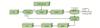 |
Fig. 1 Schematic diagram of the distributed fiber-optic vibration sensing system based on  -OTDR -OTDR
|
In practice, unauthorized intrusions such as vehicles, pedestrians, wind, and rain will cause vibration of fiber optic cables, so it is necessary to accurately determine the type of event in order to provide users with a reasonable response plan. Figure 2 illustrates a comparative presentation of data formats between the vibration location diagram and the spatiotemporal diagram within the experimental scenario. However, these events do not exhibit distinct morphological features in the X-Y spatiotemporal maps, and it is difficult to accurately differentiate between the types of signals through the spatiotemporal maps alone. In contrast, the amplitude-position plot in Fig. 2 clearly characterizes the intrusion signal in terms of spectral features, waveform morphology, and energy distribution, presenting more details. Meanwhile, compared with spatiotemporal maps, amplitude-position maps have a smaller amount of waveform curve data, a shorter training cycle, and lower storage requirements, making them more suitable for large-scale sample training. Therefore, waveform curves are selected to construct training samples in this study.
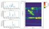 |
Fig. 2 Amplitude-position curves for (a) walking in place, (b) walk, (c) jumping in place vs. (d) spatio-temporal plots for data presentation format |
1.2 CNN, LSTM and Attention Mechanisms
A Convolutional Neural Network (CNN) is a neural network model centered on convolutional operations, where spatial features of a target are extracted by employing convolutional kernels of varying numbers and sizes[14]. Figure 2 presents the various types of amplitude-position curves that exhibit different contour patterns and amplitude characteristics, where the amplitude of each sampling point indicates the intensity of vibration at that location, and the location corresponds to the spatial distribution of the sampling points. Since the amplitudes of the sampled points are arranged in a one-dimensional sequence in chronological order, a one-dimensional convolution operation can be used to extract local features at spatial locations and further analyze the characteristics of the signal[9,15-16] . The convolution kernel slides along the amplitude-position curve, and local features are extracted through convolution operations. These features may reflect specific vibration patterns or trends in amplitude changes at a given location. More abstract and high-level feature information can be extracted through the gradual superposition of multiple convolutional layers. After the convolutional layer, pooling operations are usually introduced to reduce the dimensionality of the feature map, thus optimizing computational efficiency and reducing the complexity of the model. The pooling operation allows for maximum pooling selection. Convolutional layers can capture local features whose amplitude varies with position by stacking multiple layers. By sliding the convolution kernel, different frequency patterns, amplitude variations, peaks, periodic fluctuations, and more in the vibration signal can be identified. The features extracted by the convolution operation can identify periodic patterns, anomalous signals, as well as local peaks and troughs in the amplitude-position curve.
Figure 3(a) and (b) show the schematic diagrams of 1-D and 2-D convolution operations.
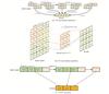 |
Fig. 3 CNN and LSTM operation process |
Long Short-Term Memory (LSTM) is a special type of recurrent neural network (RNN) that can effectively handle long-term dependencies in time-series signals.  -OTDR signals tend to be continuous time series, and LSTM can capture the temporal characteristics of event occurrences by remembering the historical states. The characteristic pulses in the
  -OTDR signal have features that are not only dependent on the input at the current moment but are also closely related to the states at previous time points. Therefore, the memory mechanism of LSTM can effectively handle this type of signal. The LSTM network processes the
  -OTDR signal through forgetting gates, which discard information about features at certain moments when they are irrelevant to the current prediction; input gates, which are responsible for introducing new impulse features in the
  -OTDR signal and updating them to the current state; and output gates, which are used for determining the LSTM outputs at each moment [11-12,16].
As shown in Fig. 3(c), the LSTM takes the sampled points within the time window as inputs, through which it generates predictions based on the window range. By setting a step-shift window, the model continuously predicts the sequence data, thus effectively extracting the time-series features of the signal.
The role of the attention mechanism is to enable the model to focus on the most important time periods or modal features, thus improving the overall recognition accuracy. For distributed fiber-optic vibration data, where the signal may contain a large amount of noise and uncorrelated parts, a Transformer-based self-attention mechanism can capture critical time steps and modal features more efficiently. The self-attention mechanism dynamically assigns weights by calculating the global correlation between time steps in the input sequence, thus helping the model to ignore unimportant parts and focus only on the most meaningful time periods or modal features[11-12,17]. Adding an attention mechanism after the output layer of the LSTM allows the model to adaptively focus on critical time steps, enhancing the recognition of important modal features. By weighted summation of the LSTM outputs, more representative features are generated for final classification[18-21].
In summary, this study utilizes the amplitude-position curve as the input for the neural network. The convolution operator extracts contour features and energy distribution characteristics from the amplitude-position curve, while the LSTM captures its time-series characteristics. By incorporating an attention mechanism, the feature expression capability is enhanced, ultimately enabling pattern recognition through feature fusion.
2 CLTNet Network Construction
2.1 Network Construction and Training
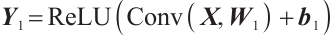
The model architecture is shown in Fig. 4. The input data to the model is shaped as a (1, 10 000,12) 3-D matrix, indicating that the data contains 1 channel, 10 000 time steps, and 12 features. For each time step t, the input data  can be represented by Eq. (1) as:
 (1)
(1)
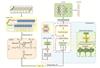 |
Fig. 4 CLTNet model network architecture diagram |
The data is first processed through two layers of convolutional operations. The main role of these layers is to start from low-level features and gradually extract more complex high-level features. The layers use the ReLU activation function as well as pooling layers to reduce the spatial dimensions between them. In the first convolutional layer, spatial features are extracted through a convolutional operation with a kernel size of (200, 3) and a stride of (50, 1), resulting in an output shaped like (5, 99, 7), which is then processed by the ReLU activation function. The operation of convolutional layer 1 can be expressed by equation (2) as:
 (2)
(2)
where  is the input,
  is the convolution kernel,
  is the bias term, and
  is the convolution operation. This is followed by downsampling the data through a maximum pooling layer to further reduce the spatial dimensionality. Additionally, a second convolutional layer is employed to further process the convolved features. The convolution kernel size is (20, 2), the stride is (4, 1), the input data shape is (5, 99, 7), 10 feature maps are output, and the spatial dimension of the data is further compressed to (10, 24, 6). The operation of Convolutional Layer 2 can be expressed by equation (3) as:
 (3)
(3)
The shape of the output feature map is  ,and the spatial features extracted by the convolutional layer need to be reshaped in order to be used as inputs to the LSTM module. In this layer, the shape of the data is reshaped from (10, 24, 6) to (batch_size, 10, 144), where 144 is the feature dimension of each time step (i.e., 24×6), providing sufficient input information for the LSTM module. The output
  of the convolutional layer is reshaped into a one-dimensional vector, which is used as the input to the subsequent LSTM module. The shape of the unfolded data is
  , where 144 is the dimension of the unfolded features. The process can be expressed by equation (4) as:
 (4)
(4)
The main task of the LSTM module is to capture the temporal dependencies in the input sequence. The input data shape of this module is (batch_size,10,144), i.e., the input for each time step is a 144-dimensional feature. The output of the LSTM is (batch_size,10,50), where 50 is the number of hidden units in the LSTM. With the multilayer structure of the LSTM, the model can effectively learn and maintain the temporal dependencies of the input sequences, overcoming the gradient vanishing problem of traditional RNNs when dealing with long sequences. The working process of the LSTM is described by the following equation:
Forget gate:
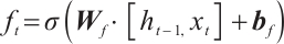 (5)
(5)
Input gate:
 (6)
(6)
Candidate memory:
 (7)
(7)
Updates the unit status:
 (8)
(8)
Output gate:
 (9)
(9)
Final hidden state:
 (10)
(10)
where  is the input of the current time step,
  is the hidden state of the previous time step,
  is the cell state of the previous time step,
  ,
,  ,
,  ,
,  and
and  ,
,  ,
,  ,
,  are the trainable parameters,
  is the Sigmoid activation function, and tanh is the hyperbolic tangent activation function.
After the LSTM module, the data is fed into the Transformer module. The Transformer module further learns the global context information in the input sequence through a self-attention mechanism. The self-attention mechanism is represented by equation (11) as:
 (11)
(11)
where  ,
,  , and
, and  are the query, key, and value matrices, respectively, and
  is the dimension of the key vector. Its main function is to capture the interrelationships among time steps in the sequence and to enhance the model's ability to perceive global information. The input to this module is the output of the LSTM with the shape (batch_size, 10, 50). The Transformer module uses a two-layer encoder (Encoder), each layer including a multi-head self-attention mechanism (with nhead=2) that computes the dependencies between different positions in parallel. The Transformer can effectively capture long-distance dependencies in sequences through its self-attention mechanism, allowing the model to more accurately handle time-series data. Each layer of the Transformer encoder is further enhanced with a feed-forward neural network for feature representation. The output of the Transformer module is (batch_size, 10, 50), i.e., the feature dimension of each time step is 50. To obtain the final classification result, the model extracts the feature representation of the last time step from the output of the Transformer, i.e., transformer_out [:, -1, :]. This step represents the global features of the time-series data sequence as input to the fully connected layer. The fully connected layer maps this feature onto six categories, and the output shape is (batch_size, 6), which is the final classification result. It can be expressed by equation (12) as:
 (12)
(12)
where  is the weight matrix of the fully connected layer,
  is the bias term, and
  is the classification result.
The output layer of the model maps the global features extracted by the Transformer to the six categorical labels through a fully connected layer. This layer utilizes the softmax activation function for classification prediction, maps the output of the network to the probability values for each category, and ultimately outputs the predicted category labels.
In the CLTNet model, the CNN, LSTM, and Transformer modules work together to achieve accurate classification of fiber-optic vibration signals. Firstly, the CNN module extracts local signal features through a one-dimensional convolution operation. Optical fiber vibration signals typically exhibit clear local patterns, such as periodic fluctuations and amplitude variations, from which CNNs effectively extract these local features. Next, the LSTM module is responsible for capturing the temporal dependencies in the signal sequence, which is critical for modelling the dynamic patterns of vibration signals over time. Finally, the Transformer module captures global information within the signal through the self-attention mechanism, enabling it to model long-range dependencies between different time steps, thus enhancing the model's ability to identify complex events.
In this study, the Adam optimizer was used during the training process, with the initial learning rate set to 0.001. A learning rate decay strategy was applied, where the learning rate was reduced to 50% of the original rate after every 10 training cycles. The batch size was set to 64, and the number of training epochs was set to 50.
All models were built and trained on AutoDL with 15 vCPUs Intel® Xeon® Platinum 8358P CPUs running at 2.60 GHz and RTX 3090 (24 GB) GPUs.
2.2 Experiments
The experiments were conducted using the distributed fiber optic vibration sensing system described in Section 2.1, whose components are shown in Fig. 5. In the experiment, the sensing fiber was buried 10 cm below the bridge gap in a surrounding environment consisting mainly of sand, some clay, and stone particles. Taking into account factors such as sensitivity and fiber optic cable strength, a suitable deployment plan was selected. In this experiment, single-mode dual-core G652D armored optical fiber was used, and FC-APC flanges were employed to connect 5 000 m bare fiber with 200 m armored optical fiber, with the experiment being conducted on the armored optical fiber.
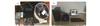 |
Fig. 5 Physical diagram of distributed fiber optic vibration sensing (a) Diagram of distributed optical fiber vibrating devices; (b) Physical diagram of distributed optical fiber integration. |
The fiber layout is depicted in Fig.6. The system captured six events: pedestrian bridge crossing signal, cycling bridge crossing signal, car bridge crossing signal, wind blowing signal, rain signal, and no intrusion status signal. The event scenario is shown in Fig.7. Each event cropped spatiotemporal signal sample consists of 10 000 points in the temporal domain and 12 neighboring spatial points in the spatial domain. The number of samples per event is detailed in Table 1. To demonstrate the dataset's utility, we conducted classification experiments on these six types of events using the CLTNet model. The training and test data were randomly selected from the dataset in an 80:20 ratio, ensuring no overlap between them.
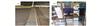 |
Fig. 6 Field fiber optic arrangement (a) Fiber layout location; (b) Location diagram of the upper computer. |
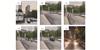 |
Fig. 7 Experimental event scenario diagram for (a) blow, (b) no-invasion state, (c) walk, (d) cycling, (e) car, and (f) rain |
Figure 8 shows the results after differentiating the cropped samples collected using a 5 200 m fiber. The value of the vertical axis represents intensity and is dimensionless. The temporal and spatial distribution patterns of events are observed to vary. Rain and wind are continuous vibration events. Due to the location of wind data collection differing from the remaining five events, the intensity changes at these points exhibit greater distinction compared with the other events. Pedestrian crossing, cycling, and car crossing events present more obvious peaks with varying peak intensities. In contrast, the no-intrusion state lacks prominent peaks and exhibits overall fluctuations of small magnitude due to background noise. To ensure the robustness of the experimental data, the wind, rain, and no-intrusion states were collected at different times.
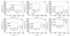 |
Fig. 8 Categorization of experimental events for (a) blow, (b) no-invasion state (c) walk, (d) cycling, (e) car, and (f) rain |
Sample size and label of the six events
2.3 Comparison and Analysis of Results
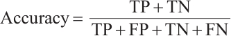
To verify the practical effectiveness of the model, we compare the proposed deep learning model with traditional methods and other advanced algorithms in the field. The expression for accuracy is shown in equation (13):
 (13)
(13)
where  is the number of samples correctly predicted to be in the positive category;
  is the number of samples incorrectly predicted to be in the positive category;
  is the number of samples incorrectly predicted to be in the negative category; and
  is the number of samples correctly predicted to be in the negative category. Figure 9 shows the confusion matrices for each of the six models: CNN+LSTM+Transformer, TAM+BiLSTM, CNN+CBAM, Wavenet, LSTM, and 1-D CNN. A comparison can be seen in Fig.9(a). In the two categories of stateless intrusion and wind blowing, the vibration signal characteristics are obvious and can be accurately identified. However, in the riding-through event, 33 samples were misclassified as pedestrians passing by. This misclassification is due to the diagnostic overlap between the two categories of vibration signals. Similarly, 22 samples were misclassified between the car passing by and rain categories, reflecting the similarity of the vibration signals. For a more intuitive understanding of the distinguishability of events, the model's features are visualized as shown in Fig.10. The final feature vector obtained from the trained model is reduced to a three-dimensional vector using the PCA algorithm, which demonstrates good differentiation ability for all six events.
 |
Fig. 9 Confusion matrix diagram for the six models |
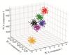 |
Fig. 10 Feature visualization Note: red, blue, purple, black, orange, and green represent labels 0, 1, 2, 3, 4, and 5, respectively. |
In this study, we conducted experiments evaluating validation accuracy and validation loss for different model architectures (CNN+LSTM+Transformer, TAM+BiLSTM, CNN+CBAM, Wavenet, LSTM, and 1-D CNN) to assess their performance in the fiber optic vibration signal pattern recognition task. The experimental results are shown in Fig.11(a) and (b), demonstrating the trends of validation accuracy and validation loss for each model over 50 training epochs.
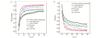 |
Fig. 11 Comparison of model accuracy (a) and validation losses (b) |
The validation accuracy of CNN+LSTM+Transformer rapidly rises above 0.85 during the early stages of training (the first 10 epochs), which is significantly higher than that of other models. This demonstrates that the model can quickly extract key features at an early stage and establish effective initial discrimination. Meanwhile, its validation loss rapidly decreases during the initial period, indicating that the model is being optimized efficiently. At the end of training, the validation accuracy of CNN+LSTM+Transformer reaches approximately 0.92, and the validation loss stabilizes around 0.20, both of which are significantly better than those of the other models. This result indicates that the CNN+LSTM+Transformer model can efficiently extract key features from fiber vibration signals and quickly establish stable classification boundaries. The low value and stability of the validation loss demonstrate that the model has good generalization ability and robustness, and can maintain high performance in complex vibration scenarios without being easily affected by background noise or signal interference. Compared with other models, CNN+LSTM+Transformer exhibits better convergence of validation loss and fluctuates less across training rounds. This stability allows it to adapt to complex backgrounds and diverse defect types, further enhancing its application potential. TAM+BiLSTM and CNN+CBAM are second only to CNN+LSTM+Transformer in terms of verification accuracy and loss. The final validation accuracy of the TAM+BiLSTM model stabilizes at 0.90, with a validation loss of 0.26. The final validation accuracy of the CNN+CBAM model stabilizes at 0.86, with a validation loss of approximately 0.31. The final validation accuracies of Wavenet and LSTM are 0.82 and 0.78, respectively, while the validation losses range from 0.50 to 0.60. TAM+BiLSTM introduces a multiple-attention mechanism (TAM), which enhances the ability to capture local keypoints of time-series data but lacks effective modeling of global dependencies. CNN+CBAM uses the channel and spatial attention module (CBAM) in the signal feature extraction stage, which improves the characterization of local features but its relative lack of temporal feature capture capability limits further performance improvement. The LSTM model mainly relies on temporal modeling and does not incorporate a spatial feature extraction module, resulting in limited ability to capture short-time local features in complex vibration signals. The validation accuracy of the 1-D CNN is only 0.73, and the validation loss is maintained above 0.65 throughout the training process, which shows the 1-D CNN performs significantly worse than other models. This disadvantage stems from the limitations of 1-D CNNs in processing multidimensional vibration signals, which are difficult to capture complex temporal features and global information and are less robust to noise.
3 Conclusion
This study systematically evaluates the performance of multiple deep learning models in fiber-optic distributed vibration measurement tasks, including CNN+LSTM+Transformer, TAM+BiLSTM, CNN+CBAM, Wavenet, LSTM, and 1-D CNN. Through experimental comparisons of validation accuracy and validation loss, the results demonstrate that the CNN+LSTM+Transformer model exhibits significant advantages in vibration signal recognition and classification, validating its potential in complex signal processing tasks.
CNN+LSTM+Transformer, with its hybrid architecture design, combines the local feature extraction capability of CNN, the temporal dynamic modeling capability of LSTM, and the global dependency capture capability of Transformer, and achieves an excellent validation accuracy of around 0.92 and a stable validation loss of 0.20. In contrast, TAM+BiLSTM and CNN+CBAM perform well in local feature extraction and temporal modeling but lack sufficient integration of global information, and their validation accuracy does not exceed 0.90. Wavenet and LSTM have some advantages in time-series data processing but lack the ability to jointly model local and global information when dealing with complex fiber vibration signals. The 1-D CNN has the worst performance and is ineffective at classifying complex vibration signals.
The CLTNet model maintains an accuracy of 0.92 despite high noise and complex backgrounds, demonstrating its robustness in practical applications. This is particularly valuable in fields such as intrusion detection and structural health monitoring, where complex environments often contain ambient noise and interfering signals. The CLTNet effectively distinguishes between useful signals and noise through its multi-module feature extraction capability, maintaining high classification accuracy even under challenging conditions. The results confirm the model's adaptability to complex scenarios and underscore its reliability in practical applications.
This paper also has certain limitations. The model exhibits high computational complexity: the hybrid architecture of CNN, LSTM, and Transformer, while improving classification accuracy, consumes a large amount of computational resources. This may become a bottleneck in real-world applications that demand high real-time performance. Future research could focus on simplifying the model structure or adopting lightweight methods to reduce computational complexity, thereby meeting real-time application requirements while ensuring accuracy.
References
- Liu Z Y, Zhang F X, Sun Z H, et al. Distributed fiber optic sensing signal recognition based on class-incremental learning[J]. Optical Fiber Technology, 2024, 87: 103940. [Google Scholar]
-
Zheng Z Y, Feng H, Sha Z, et al. A hand-crafted
 -OTDR event recognition method based on space-temporal graph and morphological object detection[J]. Optics and Lasers in Engineering, 2024, 183: 108513.
[Google Scholar]
-OTDR event recognition method based on space-temporal graph and morphological object detection[J]. Optics and Lasers in Engineering, 2024, 183: 108513.
[Google Scholar]
- Li X L, Sun Q Z, Wo J H, et al. Hybrid TDM/WDM-based fiber-optic sensor network for perimeter intrusion detection[J]. Journal of Lightwave Technology, 2011, 30(8): 1113-1120. [Google Scholar]
- Zhao S, Zhou R, Luo M M, et al. Distributed fiber optic sensing system for vibration monitoring of 3D printed bridges[J]. Optoelectronics Letters, 2025, 21(1): 28-34. [Google Scholar]
- Zhang Y L. Research on Signal Extraction and Pattern Recognition Method of Distributed Optical Fiber Vibration Sensing System[D]. Changchun: Jilin University, 2021 (Ch). [Google Scholar]
-
Wang M, Sha Z, Feng H, et al.
 -OTDR pattern recognition based on LSTM-CNN[J]. Acta Optica Sinica, 2023, 43(5): 19-30 (Ch).
[Google Scholar]
-OTDR pattern recognition based on LSTM-CNN[J]. Acta Optica Sinica, 2023, 43(5): 19-30 (Ch).
[Google Scholar]
-
Cao X M, Su Y S, Jin Z Y, et al. An open dataset of
 -OTDR events with two classification models as baselines[J]. Results in Optics, 2023, 10: 100372.
[Google Scholar]
-OTDR events with two classification models as baselines[J]. Results in Optics, 2023, 10: 100372.
[Google Scholar]
- Ma D Y, Liu X Y, Li Y Z, et al. Application progress of machine learning technology in improving the performance of distributed fiber optic sensing[J]. Progress in Laser and Optoelectronics, 2025, 62(3): 25-43 (Ch). [Google Scholar]
- Wang M S, Huang B, He C P, et al. A fault diagnosis model for complex industrial process based on improved TCN and 1D CNN[J]. Wuhan University Journal of Natural Sciences, 2022, 27(6): 453-464. [Google Scholar]
- Zhang Y, Zhao W A, Dong L L, et al. Intrusion event identification approach for distributed vibration sensing using multimodal fusion[J]. IEEE Sensors Journal, 2024, 24(22): 37114-37124. [Google Scholar]
- Liu J W, Wang Y F, Luo X L. Research Progress on Deep Memory Networks[J]. Chinese Journal of Computer Science, 2021, 44(8): 1549-1589 (Ch). [Google Scholar]
- Zou Y H, Zhang Y F, Zhao X D. Self-supervised time series classification based on LSTM and contrastive transformer[J]. Wuhan University Journal of Natural Sciences, 2022, 27(6): 521-530. [Google Scholar]
- Ma X R, Mo J Q, Zhang J W, et al. Optical fiber vibration signal recognition based on the fusion of multi-scale features[J]. Sensors, 2022, 22(16): 6012. [Google Scholar]
- Jin X B, Liu K, Jiang J F, et al. Multi-dimensional distributed optical fiber vibration sensing pattern recognition based on convolutional neural network[J]. Acta Optica Sinica, 2024, 44(1): 384-394(Ch). [Google Scholar]
- Zhu C Y, Yang K X, Yang Q M, et al. A comprehensive bibliometric analysis of signal processing and pattern recognition based on distributed optical fiber[J]. Measurement, 2023, 206: 112340. [Google Scholar]
-
Yang N C. Research on Vibration Event Detection and Identification Technology Based on
 -OTDR[D]. Zhengzhou: Information Engineering University, 2023(Ch).
[Google Scholar]
-OTDR[D]. Zhengzhou: Information Engineering University, 2023(Ch).
[Google Scholar]
- Xia Q F, Xu Y E, Li M Y, et al. A review of attention mechanisms in reinforcement learning[J]. Computer Science and Exploration, 2024, 18 (6): 1457-1475 (Ch). [Google Scholar]
- Zeng Y M, Zhang J W, Zhong Y Z, et al. STNet: A time-frequency analysis-based intrusion detection network for distributed optical fiber acoustic sensing systems[J]. Sensors, 2024, 24(5): 1570. [Google Scholar]
- Han S B, Huang M F, Li T F, et al. Deep learning-based intrusion detection and impulsive event classification for distributed acoustic sensing across telecom networks[J]. Journal of Lightwave Technology, 2024, 42(12): 4167-4176. [Google Scholar]
- Dong L L, Zhao W A, Huang S, et al. Distributed fiber optic acoustic sensing system intrusion full event recognition based on 1-D MFEWnet[J]. Physica Scripta, 2024, 99(4): 045506. [Google Scholar]
- Ma Z, Li W Z, Zhang J Z, et al. Research on feature selection algorithm for DVS vibration signal recognition rate improvement[J]. Infrared and Laser Engineering, 2024, 53(8): 238-248 (Ch). [Google Scholar]
All Tables
All Figures
|
Fig. 1 Schematic diagram of the distributed fiber-optic vibration sensing system based on -OTDR
|
| In the text | |
|
Fig. 2 Amplitude-position curves for (a) walking in place, (b) walk, (c) jumping in place vs. (d) spatio-temporal plots for data presentation format |
| In the text | |
|
Fig. 3 CNN and LSTM operation process |
| In the text | |
|
Fig. 4 CLTNet model network architecture diagram |
| In the text | |
|
Fig. 5 Physical diagram of distributed fiber optic vibration sensing (a) Diagram of distributed optical fiber vibrating devices; (b) Physical diagram of distributed optical fiber integration. |
| In the text | |
|
Fig. 6 Field fiber optic arrangement (a) Fiber layout location; (b) Location diagram of the upper computer. |
| In the text | |
|
Fig. 7 Experimental event scenario diagram for (a) blow, (b) no-invasion state, (c) walk, (d) cycling, (e) car, and (f) rain |
| In the text | |
|
Fig. 8 Categorization of experimental events for (a) blow, (b) no-invasion state (c) walk, (d) cycling, (e) car, and (f) rain |
| In the text | |
|
Fig. 9 Confusion matrix diagram for the six models |
| In the text | |
|
Fig. 10 Feature visualization Note: red, blue, purple, black, orange, and green represent labels 0, 1, 2, 3, 4, and 5, respectively. |
| In the text | |
|
Fig. 11 Comparison of model accuracy (a) and validation losses (b) |
| In the text | |
Current usage metrics show cumulative count of Article Views (full-text article views including HTML views, PDF and ePub downloads, according to the available data) and Abstracts Views on Vision4Press platform.
Data correspond to usage on the plateform after 2015. The current usage metrics is available 48-96 hours after online publication and is updated daily on week days.
Initial download of the metrics may take a while.