| Issue |
Wuhan Univ. J. Nat. Sci.
Volume 31, Number 1, February 2026
|
|
|---|---|---|
| Page(s) | 45 - 57 | |
| DOI | https://doi.org/10.1051/wujns/2026311045 | |
| Published online | 06 March 2026 | |
Deep Learning and Intelligent Perception
CLC number: TP368.2
OP-SLAM: An RGB-D SLAMMOT Method Leveraging the Constraints of Object Planar Features
OP-SLAM:一种融合物体平面特征约束的RGB-D SLAMMOT方法
1
GNSS Research Center, Wuhan University, Wuhan 430072, Hubei, China
(武汉大学 卫星导航定位技术研究中心,湖北 武汉 430072)
2
School of Geodesy and Geomatics, Wuhan University, Wuhan 430072, Hubei, China
(武汉大学 测绘学院,湖北 武汉 430072)
3
School of Electronic Information, Wuhan University, Wuhan 430072, Hubei, China
(武汉大学 电子信息学院,湖北 武汉 430072)
4
Artificial Intelligence Institute, Wuhan University, Wuhan 430072, Hubei, China
(武汉大学 人工智能研究院,湖北 武汉 430072)
† Corresponding author. E-mail: This email address is being protected from spambots. You need JavaScript enabled to view it.
Received:
10
October
2025
Abstract
By integrating self-localization, environment mapping, and dynamic object tracking into a unified framework, visual simultaneous localization and mapping with multiple object tracking (SLAMMOT) enhances decision-making and interaction capabilities in applications such as autonomous driving, robotic navigation, and augmented reality. While numerous outstanding visual SLAMMOT methods have been proposed, the majority rely only on point features, overlooking the abundant and stable planar features in artificial objects that can provide valuable constraints. To address this limitation, we propose OP (object planar) -SLAM, an RGB-D SLAMMOT system that leverages planar features to improve object pose estimation and reconstruction accuracy. Specifically, we introduce an accurate object planar feature extraction and association method using normal images, alongside a novel object bundle adjustment framework that incorporates planar constraints for enhanced optimization. The proposed system is evaluated on both synthetic and public real-world datasets, including Oxford multimotion dataset (OMD) and KITTI tracking dataset. Especially on the OMD, where planar features are prominent, our method improves object pose estimation accuracy by approximately 60%. Extensive experiments demonstrate its effectiveness in enhancing object pose estimation and reconstruction, achieving notable performance compared with existing methods. Furthermore, OP-SLAM runs in real time, making it suitable for practical robots and augmented reality applications.
摘要
视觉SLAMMOT(同时定位与建图与多目标跟踪)将自定位、环境建图和动态物体跟踪集成于统一框架,在自动驾驶、机器人导航和增强现实等应用中提升决策与交互能力。尽管已有多种优秀的视觉SLAMMOT方法,但它们大多数仅依赖点特征,忽略了人工物体中丰富且稳定的平面特征,而这些特征可提供宝贵的约束信息。为解决这一局限,本文提出OP-SLAM,一种利用平面特征提升物体位姿估计与重建精度的RGB-D SLAMMOT系统。具体而言,我们基于法向图像提出了精确的物体平面特征提取与关联方法,并设计了一种融合平面约束的新型物体捆集调整框架以增强优化效果,所提出的方法在合成数据集及公开真实数据集(包括OMD和KITTI tracking)上进行了验证。大量实验结果表明,该方法在物体位姿估计与重建方面均取得了显著效果,并优于现有方法。尤其是在平面特征显著的OMD数据集上,我们的方法将物体位姿估计精度提升约60%。此外,OP-SLAM可实时运行,适用于实际机器人和增强现实应用。
Key words: visual simultaneous localization and mapping (SLAM) / multiple object tracking (MOT) / dynamic scenes / planar feature
关键字 : 视觉SLAM / 多目标跟踪 / 动态场景 / 平面特征
Cite this article:WANG Yingli, LIU Yang, GUO Chi. OP-SLAM: An RGB-D SLAMMOT Method Leveraging the Constraints of Object Planar Features[J]. Wuhan Univ J of Nat Sci, 2026, 31(1): 45-57.
Biography: WANG Yingli, female, Master candidate, research direction: dynamic VSLAM and robot navigation. E-mail: This email address is being protected from spambots. You need JavaScript enabled to view it.
Foundation item: Supported by Major Science and Technology Project of Hubei Province (2022AAA009)
© Wuhan University 2026
 This is an Open Access article distributed under the terms of the Creative Commons Attribution License (https://creativecommons.org/licenses/by/4.0), which permits unrestricted use, distribution, and reproduction in any medium, provided the original work is properly cited.
0 Introduction
Visual simultaneous localization and mapping (SLAM) is a technology that enables a vision sensor-equipped platform to simultaneously localize itself and construct a map of an unknown environment. It has long been a foundational technology in computer vision[1] and has evolved into a critical and highly active research area over the years, with notable advancements such as ORB-SLAM[2] and VINS-mono[3].
Most traditional visual SLAM methods rely on the static scene assumption, which presumes that changes between consecutive frames are solely attributed to camera motion. However, real-world environments are often populated with dynamic objects, which can introduce errors in camera pose estimation. To address this issue, some methods employ the RANSAC (RANdon SAmples Consensus) strategy to identify and eliminate outlier points[4], while others focus on detecting movable objects and rejecting the dynamic points associated with them[5-6]. Nevertheless, the pose, motion trend, and other information of dynamic objects are crucial for tasks such as target tracking and obstacle avoidance. As a result, recent methods have sought to integrate visual SLAM with multiple object tracking (MOT), commonly referred to as visual simultaneous localization and mapping with multiple object tracking (SLAMMOT)[7-8]. Specifically, SLAM provides real-time self-pose estimation, ensuring an updated coordinate system for dynamic object tracking. In turn, MOT compensates for SLAM's limitations under the static scene assumption by providing motion cues that help SLAM distinguish static from dynamic elements or by tightly optimizing camera poses, improving localization accuracy and stability.
Currently, visual SLAMMOT methods predominantly use point features. However, real-world environments often exhibit abundant and stable planar features, which can be used to enhance localization and mapping accuracy[9-10]. Despite the potential of planar features, their use is still restricted to static environments, such as utilizing walls and floor to improve camera pose accuracy[11]. Their application in dynamic object pose estimation, however, remains largely unexplored.
In this study, we propose an RGB-D SLAMMOT system that incorporates planar features from object surfaces in addition to traditional point features, as shown in Fig. 1(a). These planar features are used to construct relevant constraints, improving both object pose estimation and reconstruction accuracy. This supports applications such as augmented reality (AR) and robotic interaction, which require precise dynamic object tracking and surface reconstruction, as demonstrated in Fig. 1(b). The main contributions of this study are as follows:
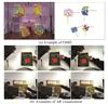 |
Fig. 1 Output of our system (a) Planes extracted from dynamic objects, color-coded for differentiation. (b) AR examples demonstrating how our method stably anchors a virtual object onto the real surface of a freely moving dynamic object. |
• An accurate object planar feature extraction and association method using normal images.
• A novel object bundle adjustment framework that integrates planar constraints for enhanced optimization.
Experiments demonstrate that our proposed method improves the accuracy of object pose estimation and reconstruction.
1 Related Work
A variety of methods have been proposed to improve the accuracy and robustness of RGB-D SLAM. Some focus on system-level enhancements such as calibration, loop closure, and graph optimization[12], while others address dynamic objects or exploit high-level primitives like planes.
1.1 Visual SLAMMOT
Unlike some dynamic visual SLAM methods that segment and filter out dynamic portions of the scene, such as DS-SLAM[5] and DynaSLAM[6], visual SLAMMOT methods focus on detecting and tracking dynamic objects. CubeSLAM[13] generates 3D bounding boxes from 2D ones using vanishing points, incorporating object priors such as vehicle dimensions and road structures. ClusterVO[14] clusters point clouds for probabilistic data association and jointly optimizes camera and object poses within a sliding window. VDO-SLAM[15] employs dense optical flow for feature tracking and jointly optimizes the flow results with object poses. DynaSLAM Ⅱ[16] adopts an object-dominant optimization strategy, reducing parameters and jointly optimizing camera and dynamic object states within a bundle adjustment (BA) framework. TwistSLAM[17] enhances vehicle pose estimation accuracy by incorporating road surface constraints. AirDOS[18] explores rigid-body constraints by decomposing the human body into keypoints and connecting rods, estimating poses through factor graph optimization. Recent advancements include Yang et al[19], which improves the robustness and accuracy of multi-object state estimation by integrating motion priors, road surface constraints, and uncertainty modeling. DynaMeshSLAM[8] employs a mesh to reconstruct object surfaces and builds deformation graphs for optimizing both mappoints and object poses. DMOT-SLAM[20] is a SLAMMOT system suitable for both indoor and outdoor dynamic environments, which achieves precise dynamic region partitioning and enables semi-dense semantic map construction. SDPL-SLAM[21] incorporates static and dynamic points and lines, introducing novel line segment correspondences and error terms to enhance pose estimation accuracy. DynoSAM[22] is a dynamic SLAM framework that integrates factor graph-based smoothing and mapping approaches to provide a robust solution for multi-object tracking and mapping problems. These methods collectively demonstrate the growing emphasis on leveraging dynamic information to improve the accuracy and utility of visual SLAM systems in complex, real-world environments. However, all of the methods mentioned above ignore the object planar features, which can be used to improve object pose estimation and reconstruction.
1.2 Planar SLAM
Rich and stable planar features in real-world environments can significantly enhance the localization and mapping accuracy of SLAM systems. For instance, Salas-Moreno et al[23] proposed a dense SLAM system capable of detecting and modeling bounded planar regions commonly found in artificial scenes. Ma et al[24] incorporated planar constraints into pose estimation for the current frame and refine keyframe poses and global planes during global graph optimization to ensure consistency. Hsiao et al[25] introduced a keyframe-based dense planar SLAM, which achieves accurate relative pose estimation through correct plane correspondences between frames and generates a globally consistent planar map. Rosinol et al[11] leveraged a 3D mesh representation to detect and enforce vertical or horizontal planar constraints. Li et al[9] proposed a novel visual-inertial-plane PnP algorithm for fast localization, introducing a structureless plane-distance cost in sliding-window optimization. Their subsequent work[26] employed a plane instance segmentation network to detect planar regions, refine these regions by extracting 2D point and line features from images, and leverage co-planar relationship to improve camera pose accuracy. Xing et al[27] proposed an RGB-D visual odometry method that jointly utilizes point, line, plane, and Manhattan features with depth uncertainty modeling and local bundle adjustment, leading to improved pose accuracy and robustness. To address the scarcity of point features in dynamic environments, some methods, such as proposed by Ram et al[10] and Wang et al[28], augment SLAM systems with planar features. While all the aforementioned methods focus on utilizing static planes in the environment, planar features are often abundant on artificial objects as well. Long et al[29] tackled this by separating dynamic planar objects based on their rigid motions, enabling localization and tracking without semantic cues, which reduces computational overhead and avoids segmentation failures. In contrast, our method combines semantic and geometric information, which can improve object recognition and tracking accuracy.
2 System Overview and Notation
2.1 System Overview
The overview of our pipeline is illustrated in Fig. 2. Our system takes RGB-D images as input. Instance segmentation[30] and normal image[31] are acquired respectively to prepare for the object tracking. The pipeline is mainly composed of two components: camera pose estimation with static mapping and object pose estimation with dynamic reconstruction. In the first component, potential outliers caused by dynamic objects are filtered during point feature extraction. After feature tracking, the camera pose is estimated by minimizing the reprojection error and then refined through local map optimization. In the second component, instance segmentation masks are used to associate objects between frames, followed by feature tracking and initial pose estimation for the associated objects. Then, object planar features are extracted using normal images and associated based on feature correspondences and plane parameters. After that, an optimization framework incorporating planar features is used to further optimize the initial object pose. Finally, we can construct a map consisting of camera poses, static mappoints, object poses, dynamic mappoints, and dynamic planes.
 |
Fig. 2 Overview of the OP-SLAM system Note: The framework of the OP-SLAM system is composed two core modules: camera pose estimation with static mapping, and object pose estimation with dynamic reconstruction. The system integrates these processes to generate a map. The subfigures in the diagram represent the data used: (a) RGB image, (b) depth image, (c) segmentation mask, and (d) normal image. |
2.2 Notation
2.2.1 Coordinate system
The coordinate systems involved in this study mainly include the world coordinate system  , the camera coordinate system
  , and the object coordinate system
  . The world coordinate system coincides with the camera coordinate system of the first frame. For each object, its coordinate system is established independently of the extracted planar features: the initial axes are aligned with those of the camera coordinate system that first observes the object, and the initial origin is set at the center of the object's initialized point cloud.
2.2.2 Pose representation
The camera pose of the  -th frame can be expressed as
 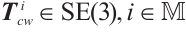 , where
  denotes camera frame indices set, and
  represents the group of rigid-body transformations in 3D space. Similarly, the pose of the
  -th object in the
  -th frame is represented as
  , where
  denotes object indices set.
2.2.3 Feature representation
For point features, 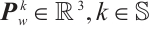 represents the coordinates of the mappoint
  in the world coordinate system, where
  denotes static mappoint indices set. The pixel coordinates of its corresponding feature in the
  -th frame are denoted as
 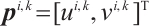 . The projection process is expressed as
  , where
  is the projection function. For planar features, we adopt the Hesse form to describe them. For example, a plane in the object coordinate system is represented as
  , where
  is the normal vector of the plane in the object coordinate system,
  denotes the signed distance from the object coordinate origin to the plane, and
  is object plane indices set. A point feature
  lying on the plane satisfies
  . However, planes in 3D space have only three degrees of freedom. Using the Hesse form with four parameters results in an over-parameterization issue. To address this, we employ spherical coordinates to represent the plane during optimization, i.e.,
  , where
  is the elevation angle and
  is the azimuth angle.
3 Methods
3.1 Camera Pose Estimation with Static Mapping
To estimate the camera pose, we first extract Shi-Tomasi features[32] from the image. To improve the accuracy of camera pose estimation, keypoints within the masks of potentially dynamic objects are excluded, and only features from static regions are retained. Next, the Lucas-Kanade (LK) optical flow method[33] is employed to track these keypoints across consecutive frames. After keypoint tracking, the correspondences between existing static mappoints and the keypoints in the  -th camera frame are established, enabling the formulation of the reprojection error as follows:
 (1)
(1)
Then, the camera pose can be estimated by minimizing the objective function:
 (2)
(2)
where  is the static mappoint indices set corresponding to the keypoints in the
  -th frame, and
  is the constant covariance matrix.
To reduce pose accumulation errors and ensure the local consistency of static mappoints, a sliding window is constructed to perform local BA, optimizing camera poses and static mappoints positions. The sliding window with a constant number of frames can be divided into two parts: the inactive part and the active part. The inactive part contains older frames, which can provide constraints, while the active part contains newer frames, which are optimized in the local BA. The objective function in the camera local BA is as follows:
 (3)
(3)
where  and
and  are frame and static mappoint indices set in the active part of the sliding window respectively, and
  is frame indices set in the whole sliding window.
3.2 Object Pose Estimation with Dynamic Reconstruction
3.2.1 Object association
To associate objects, we first calculate the Intersection over Union (IoU) between instance segmentation masks of the current frame and those of the previous frame to construct a cost matrix. The optimal matching pairs are then determined using the Kuhn-Munkres (KM) algorithm[34]. To ensure a sufficient number of keypoints for object pose estimation and reconstruction, keypoints are uniformly sampled based on the object size. Once the object association relationships are established, the LK optical flow method is used to determine keypoint correspondences. Additionally, keypoints are validated to ensure they lie within the matched object masks, thereby improving the reliability of the association results. To further enhance robustness, we mitigate the effects of depth noise by filtering out keypoints with extreme depth values and applying the radius-based filter.
3.2.2 Pose estimation for dynamic objects
When estimating the poses of dynamic objects, we assume that each object is rigid, meaning that the positions of its mappoints remain relatively fixed in the object coordinate system. With the object mappoints and their corresponding keypoint pixel coordinates, the reprojection error term for an object mappoint is formulated as follows:
 (4)
(4)
The object pose can then be obtained by minimizing the objective function as follows:
 (5)
(5)
where  is the dynamic mappoint indices set of the
  -th object corresponding to the keypoints in the
  -th frame, and
  is the constant covariance matrix.
3.2.3 Object planar feature extraction and association
Normal vectors characterize the local orientation of a surface at each point, offering valuable insights into the geometric properties of the surface. As a result, normal estimation serves as a critical foundation for object planar feature extraction and association.
To extract object planar features, we adopt the algorithm detailed in Algorithm 1. Planar feature extraction is performed within the mask of each segmented object, which ensures that the extracted planes are associated with the corresponding object instance. The procedure begins by randomly selecting an object keypoint as a seed point and iteratively expanding the planar region by comparing the similarity of normal vectors. During expansion, the normal vector of the plane is continuously updated to reflect the growing region. The process continues until no more keypoints satisfy the similarity condition. The above procedure is repeated to extract multiple object planes until the remaining keypoints are insufficient. In cases where object planar features are absent or fragmented, our method avoids extracting unreliable ones.
Once the set of planar keypoints and the normal vector  are identified, the signed distance from the plane to the origin of the camera coordinate system
  is calculated as follows:
 (6)
(6)
where  is the center of the point cloud in the camera coordinate system corresponding to the planar keypoints set. Thus, the plane parameters in the camera coordinate system are obtained as
  .
.
When a plane is first observed, it can be initialized by transforming it from the camera coordinate system to the object coordinate system:
 (7)
(7)
The KM algorithm is employed for object planar feature association. The cost function in this case is based on the number of matched keypoint pairs between the newly extracted and the existing object planes. Since the matching relationships of keypoints reflect the plane correspondence to a certain extent, and homonymous points ideally lie on the same plane, this method facilitates accurate planar feature association. To suppress erroneous matches, we further introduce a motion-compensated geometric verification. Specifically, each plane from the previous frame is propagated into the current camera coordinate system using the estimated camera motion, yielding its predicted parameters. An association is considered valid only when the detected plane's normal orientation and offset agree with the propagated parameters within predefined thresholds; otherwise, the association is discarded. If a newly extracted plane fails to associate with any existing plane, a new plane is initialized as described in Eq. (7).
| Algorithm 1 Object plane extraction |
|---|
Input:
 - Keypoints set of object - Keypoints set of object  in the in the  -th frame, -th frame,  - Normal image of the - Normal image of the  -th frame, -th frame,  - Camera intrinsic matrix - Camera intrinsic matrix |
Output:
 - Planar feature set of object - Planar feature set of object  in the in the  -th frame -th frame |
0:  , , 
|
1: while Size ( ) )  do do
|
2: 
|
3: 
|
4: 
|
5: for all  in { in { } do } do
|
6: 
|
7: if  then then
|
8: 
|
9: Add  to to 
|
| 10: end if |
| 11: end for |
12: Remove  from from 
|
13: if Size ( ) )  then then
|
14: 
|
15: 
|
16: 
|
17: Add  to to 
|
| 18: end if |
| 19: end while |
3.2.4 Object planar constraints
Once object planar feature extraction and association are completed, the extracted object planes are used to construct planar constraints, namely the point-to-plane constraint and the plane-to-plane constraint, as illustrated in Fig. 3. Considering the structural characteristics of the object surface, points lying on a plane ideally have zero distance to it, i.e., they satisfy  . However, this ideal condition is hardly perfectly met in practice. To address this, a point-to-plane error term is formulated to enhance the accuracy of object surface reconstruction and pose estimation:
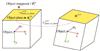 |
Fig. 3 3D illustration of the planar error terms, specifically the point-to-plane error term and plane-to-plane error term |
 (8)
(8)
Moreover, since planar features are derived from multiple points, they tend to retain greater stability even when individual points are affected by noise, making them inherently resistant to such disturbances. As a result, the inter-frame plane association relationships provide reliable information for object pose estimation. To leverage this, we formulate the plane-to-plane error term as follows:
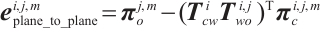 (9)
(9)
3.2.5 Object local BA with planar constraints
After the initial object pose estimation, the object pose is further optimized in the local map. This method, which separates the BA optimization of the camera and the object, as in DynaMeshSLAM[8], mitigates the mutual interference between the initial rough poses and improves the efficiency of the overall optimization solution. In addition to the object mappoint reprojection error term, the optimization incorporates the object constant velocity error term, as well as the point-to-plane and plane-to-plane error terms. These error terms are integrated into a factor graph for object BA, as illustrated in Fig. 4.
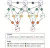 |
Fig. 4 The factor graph corresponding to the object local BA |
Considering the smooth motion of the object and the absence of significant positional jumps, an object constant velocity error term is introduced to ensure the accuracy of the object pose estimation:
 (10)
(10)
where  is the mapping from a Lie group to its Lie algebra, and
  is the motion of object
  from the
  -th frame to the
  -th frame.
Finally, the overall objective function of object BA optimization is formulated as follows:
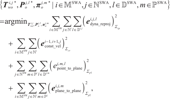 (11)
(11)
where  ,
,  , and
, and  are the corresponding covariance matrices.
4 Experiments
4.1 Experiments Setup
We conduct three experiments in this article to comprehensively validate the performance of our proposed method. The first experiment uses a synthetic dataset generated with Isaac Sim[35], which offers a controlled environment for demonstrating plane association and conducting an ablation study on planar constraints. The second experiment is performed on the public Oxford multimotion dataset (OMD)[36], which is captured with real-world sensors and contains rich planar features and diverse dynamic-object motions, making it suitable for evaluating our plane extraction method and comparing our system with existing visual SLAMMOT approaches. The third experiment is conducted on the KITTI tracking dataset[37], which provides real-world driving scenarios for further assessing object tracking and pose estimation accuracy, thereby demonstrating the generalization capability of our method.
For quantitative evaluation, we employ Absolute Translation Error (ATE) and Relative Pose Error ( )[38], where the RPE is further decomposed into translational (
 ) and rotational (
 ) components. In addition, we report the 2D True Positive Rate (2D-TP) for object tracking.
4.2 Synthetic Dataset
To validate the effectiveness of the proposed planar constraints, we used Isaac Sim to create a warehouse environment and generate five sequences, as listed in the first column of Table 1. The first four sequences each contain two cubes, where cube 0 moves along the cross, and cube 1 follows a spiral upward motion. cube_3dof indicates pure translation, while cube_6dof includes rotation. cam_static refers to a static camera, and cam_moving refers to a camera moving along the cross. The last sequence simulates a more realistic warehousing scenario, where two robots transport cartons. Robot 0 moves along a straight line, while robot 1 turns right along a curve, with the camera turning left. RGB images, depth, and instance segmentation masks were generated by the renderer. To better simulate real-world sensor measurements, Gaussian white noise with a standard deviation of 5 cm was added to the depth data. Representative examples from these sequences are shown in Fig. 5.
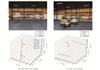 |
Fig. 5 Image and the motion trajectories of the camera and objects from partial sequences of the synthetic dataset |
The extraction and association results of object planar features are shown in Fig. 6. The results demonstrate that the planes are accurately extracted, capturing the object's geometric structure. Besides, with each object plane consistently assigned a unique color across frames, it is evident that the plane association remains stable and accurate throughout multiple frames under the six degrees of freedom motion of the objects.
 |
Fig. 6 Object planar extraction and association results on the synthetic dataset cube_6dof_cam_moving sequence Note: The red points indicate current static features. Same-colored points within an object region indicate the same plane. The blue points and black points respectively represent the estimated and ground truth trajectories of the object. |
We performed four sets of experiments for each sequence: w/o planar constraints, w/ point-to-plane constraint, w/ plane-to-plane constraint, and w/ two planar constraints. Since object local BA optimization does not affect the camera pose, we focused on comparing the object pose accuracy for each mode. The results in Table 1 indicate that the availability of point features still ensures the functionality of our system in the absence of planar constraints. However, the addition of planar constraints to object local BA improves most of the metrics across the five sequences. Further analysis reveals that the plane-to-plane constraint has a more significant benefit compared with the point-to-plane constraint. This is because the plane-to-plane constraint aligns the object surface by adjusting its pose, providing direct geometric measurement information for object pose estimation, whereas the point-to-plane constraint optimizes the object pose by adjusting the positions of the object mappoints. Besides, the planar constraints have a more pronounced effect on reducing  . This can be attributed to the fact that the normal vector of the object plane encodes orientation information. The accurate normal vector estimated by our method provides an additional constraint for object pose estimation, thereby improving the accuracy of object rotation. For more complex motion scenarios like cube_6dof_cam_moving or more realistic environments like box_cam_moving, adding planar constraints all achieves comparable or better accuracy in object pose estimation.
Object pose estimation results in different object planar constraint modes on the synthetic dataset
4.3 Oxford Multimotion Dataset (OMD)
The OMD captures multi-motion scene data from real-world environments using a device equipped with multiple sensors, including an RGB-D camera and inertial measurement unit (IMU). Additionally, a Vicon motion capture system is employed to provide ground truth trajectories for the camera and each moving object, facilitating the evaluation of multi-motion estimation techniques. For our experiments, we selected the swinging_4_unconstrained sequence, which features four boxes exhibiting distinct motion patterns. To ensure comparability with existing methods including ClusterVO, VDO-SLAM, SDPL-SLAM, and DynoSAM, we used the first 500 frames of this sequence.
The comparison of plane extraction methods is conducted on the OMD, which provides data collected from real-world environments using actual sensors. This makes it more representative of the challenges encountered in practical applications. The comparison results are shown in Fig. 7. Since existing plane extraction methods (Fig. 7(a-c)) rely heavily on depth precision, they tend to struggle in scenarios where depth measurement errors are significant. Specifically, CAPE[39] struggles to extract small-area planes on objects, while PCL's RANSAC[40] and mesh-based region growing suffer from over-segmentation issues. In contrast, our method (Fig. 7(d)) mitigates these issues by first estimating normals using a deep learning approach and then extracting planes based on normal similarity, leading to improved completeness and accuracy.
 |
Fig. 7 Qualitative comparison of planar feature extraction methods across different methods on the OMD swinging_4_unconstrained sequence |
Table 2 presents the  comparison results for both camera and object pose estimation. Compared with existing methods, our method achieves comparable accuracy in camera pose estimation but demonstrates significantly better performance in object pose estimation. Specifically, compared with the latest method, SDPL-SLAM, which leverages line features, our method reduces the average
  and
and  for the four objects by 60.0% and 62.6%, respectively. This improvement can be attributed to two key factors. First, our method exploits the surface planar properties of the object to optimize the positions of object mappoints, which, in turn, enhances the object pose estimation. The improvement is particularly pronounced in the case of noisy depth measurements, like those on the OMD. Second, as a surface structural feature, the object planar feature is relatively stable and less sensitive to noise. Their inter-frame associations further provide additional useful information, enhancing the accuracy of object pose estimation.
Camera and object pose estimation results compared with other visual SLAMMOT methods on the OMD swinging_4_unconstrained sequence
4.4 KITTI Tracking Dataset
Although our method is designed for indoor RGB-D scenarios, we conducted experiments on the KITTI tracking dataset to thoroughly evaluate its applicability. The KITTI tracking dataset offers real-world urban driving sequences with annotated object trajectories, stereo images, and LiDAR scans, serving as a standard benchmark for evaluating multi-object tracking in SLAM. Since it only provides stereo images, we employed a simple sparse stereo feature matching approach to estimate depth.
Table 3 presents a comparative evaluation of object pose estimation accuracy across different visual SLAMMOT methods on the KITTI tracking dataset. The results demonstrate that our method performs effectively on this dataset, achieving high-precision vehicle pose estimation. In certain sequences, our method attains  metrics comparable to state-of-the-art methods. However, the improvements in
  and
and  are limited. This performance limitation primarily stems from the reliance on sparse depth estimation from stereo images and the absence of road surface constraints[17,19] for driving scenarios. As for 2D-TP, our method employs a simpler association strategy and ignores distant objects, resulting in relatively lower metrics compared with Yang et al[19], but with a trade-off for higher efficiency.
As mentioned above, the primary strength of our method lies in indoor applications, particularly in AR and robotic interaction as shown in Fig. 1(b). We also plan to expand and improve our method for outdoor scenarios in future work.
Object pose estimation results compared with other visual SLAMMOT methods on the KITTI tracking dataset
5 Conclusion
In this article, we propose OP-SLAM, an RGB-D SLAMMOT system with object planar features. Considering the structural properties of the object surface and the stability of the planar features, we propose an accurate object planar feature extraction and association method, upon which we construct two planar constraints: point-to-plane and plane-to-plane. These constraints are incorporated into the object BA to further optimize object pose and improve reconstruction accuracy. Experimental results demonstrate that our method offers certain advantages in the accuracy of object pose estimation and reconstruction and achieves impressive performance.
Nevertheless, OP-SLAM may have certain limitations for non-rigid or complex-shaped dynamic objects. In future work, we aim to enhance its generalization capability and expand its applicability to practical scenarios, such as AR/VR and robotic navigation.
References
- Smith R C, Cheeseman P. On the representation and estimation of spatial uncertainty[J]. The International Journal of Robotics Research, 1986, 5(4): 56-68. [Google Scholar]
- Mur-Artal R, Montiel J M M, Tardós J D. ORB-SLAM: A versatile and accurate monocular SLAM system[J]. IEEE Transactions on Robotics, 2015, 31(5): 1147-1163. [CrossRef] [Google Scholar]
- Qin T, Li P L, Shen S J. VINS-mono: A robust and versatile monocular visual-inertial state estimator[J]. IEEE Transactions on Robotics, 2018, 34(4): 1004-1020. [CrossRef] [Google Scholar]
- Mur-Artal R, Tardós J D. ORB-SLAM2: An open-source SLAM system for monocular, stereo, and RGB-D cameras[J]. IEEE Transactions on Robotics, 2017, 33(5): 1255-1262. [CrossRef] [Google Scholar]
- Yu C, Liu Z X, Liu X J, et al. DS-SLAM: A semantic visual SLAM towards dynamic environments[C]//2018 IEEE/RSJ International Conference on Intelligent Robots and Systems (IROS). New York: IEEE, 2018: 1168-1174. [Google Scholar]
- Bescos B, Fácil J M, Civera J, et al. DynaSLAM: Tracking, mapping, and inpainting in dynamic scenes[J]. IEEE Robotics and Automation Letters, 2018, 3(4): 4076-4083. [Google Scholar]
- Lin K H, Wang C C. Stereo-based simultaneous localization, mapping and moving object tracking[C]//2010 IEEE/RSJ International Conference on Intelligent Robots and Systems. New York: IEEE, 2010: 3975-3980. [Google Scholar]
- Liu Y, Guo C, Luo Y R, et al. DynaMeshSLAM: A mesh-based dynamic visual SLAMMOT method[J]. IEEE Robotics and Automation Letters, 2024, 9(6): 5791-5798. [Google Scholar]
- Li J Y, Yang B B, Huang K, et al. Robust and efficient visual-inertial odometry with multi-plane priors[C]//Pattern Recognition and Computer Vision. Cham: Springer-Verlag, 2019: 283-295. [Google Scholar]
- Ram K, Kharyal C, Harithas S S, et al. RP-VIO: Robust plane-based visual-inertial odometry for dynamic environments[C]//2021 IEEE/RSJ International Conference on Intelligent Robots and Systems (IROS). New York: IEEE, 2021: 9198-9205. [Google Scholar]
- Rosinol A, Sattler T, Pollefeys M, et al. Incremental visual-inertial 3D mesh generation with structural regularities[C]//2019 International Conference on Robotics and Automation (ICRA). New York: IEEE, 2019: 8220-8226. [Google Scholar]
- Xu P, Su K H, Hong C, et al. Simultaneous localization and mapping technology based on project tango[J]. Wuhan University Journal of Natural Sciences, 2019, 24(2): 176-184. [Google Scholar]
- Yang S C, Scherer S. CubeSLAM: Monocular 3-D object SLAM[J]. IEEE Transactions on Robotics, 2019, 35(4): 925-938. [Google Scholar]
- Huang J H, Yang S, Zhao Z S, et al. ClusterSLAM: A SLAM backend for simultaneous rigid body clustering and motion estimation[C]//2019 IEEE/CVF International Conference on Computer Vision (ICCV). New York: IEEE, 2019: 5874-5883. [Google Scholar]
- Zhang J, Henein M, Mahony R, et al. VDO-SLAM: A visual dynamic object-aware SLAM system[EB/OL]. [2020-05-22]. arXiv:2005.11052. [Google Scholar]
- Bescos B, Campos C, Tardós J D, et al. DynaSLAM Ⅱ: Tightly-coupled multi-object tracking and SLAM[J]. IEEE Robotics and Automation Letters, 2021, 6(3): 5191-5198. [Google Scholar]
- Gonzalez M, Marchand E, Kacete A, et al. TwistSLAM: Constrained SLAM in dynamic environment[J]. IEEE Robotics and Automation Letters, 2022, 7(3): 6846-6853. [Google Scholar]
- Qiu Y H, Wang C, Wang W S, et al. AirDOS: Dynamic SLAM benefits from articulated objects[C]//2022 International Conference on Robotics and Automation (ICRA). New York: IEEE, 2022: 8047-8053. [Google Scholar]
- Yang L H, Zhang Y Z, Tian R, et al. Fast, robust, accurate, multi-body motion aware SLAM[J]. IEEE Transactions on Intelligent Transportation Systems, 2024, 25(5): 4381-4397. [Google Scholar]
- Wang K S, Yao X F, Ma N F, et al. DMOT-SLAM: Visual SLAM in dynamic environments with moving object tracking[J]. Measurement Science and Technology, 2024, 35(9): 096302. [Google Scholar]
- Manetas A, Mermigkas P, Maragos P. SDPL-SLAM: Introducing lines in dynamic visual SLAM and multi-object tracking[C]//2024 IEEE/RSJ International Conference on Intelligent Robots and Systems (IROS). New York: IEEE, 2024: 7893-7899. [Google Scholar]
- Morris J, Wang Y, Kliniewski M, et al. DynoSAM: Open-source smoothing and mapping framework for dynamic SLAM[EB/OL]. [2025-01-21]. arXiv:2501.11893. [Google Scholar]
- Salas-Moreno R F, Glocken B, Kelly P H J, et al. Dense planar SLAM[C]//2014 IEEE International Symposium on Mixed and Augmented Reality (ISMAR). New York: IEEE, 2014: 157-164. [Google Scholar]
- Ma L N, Kerl C, Stückler J, et al. CPA-SLAM: Consistent plane-model alignment for direct RGB-D SLAM[C]//2016 IEEE International Conference on Robotics and Automation (ICRA). New York: IEEE, 2016: 1285-1291. [Google Scholar]
- Hsiao M, Westman E, Zhang G F, et al. Keyframe-based dense planar SLAM[C]//2017 IEEE International Conference on Robotics and Automation (ICRA). New York: IEEE, 2017: 5110-5117. [Google Scholar]
- Li X, Li Y Y, Örnek E P, et al. Co-planar parametrization for stereo-SLAM and visual-inertial odometry[J]. IEEE Robotics and Automation Letters, 2020, 5(4): 6972-6979. [Google Scholar]
- Xing J, Zhong Q X, Liu J. Robust depth-verified RGB-D visual odometry with structural regularities for indoor environments[J]. Measurement Science and Technology, 2024, 35(3): 035407. [Google Scholar]
- Wang Y N, Xu K, Tian Y B, et al. DRG-SLAM: A semantic RGB-D SLAM using geometric features for indoor dynamic scene[C]//2022 IEEE/RSJ International Conference on Intelligent Robots and Systems (IROS). New York: IEEE, 2022: 1352-1359. [Google Scholar]
- Long R, Rauch C, Zhang T W, et al. RGB-D SLAM in indoor planar environments with multiple large dynamic objects[J]. IEEE Robotics and Automation Letters, 2022, 7(3): 8209-8216. [Google Scholar]
- Bolya D, Zhou C, Xiao F Y, et al. YOLACT: Real-time instance segmentation[C]//2019 IEEE/CVF International Conference on Computer Vision (ICCV). New York: IEEE, 2019: 9156-9165. [Google Scholar]
- Yin W, Zhang C, Chen H, et al. Metric3D: Towards zero-shot metric 3D prediction from a single image[C]//2023 IEEE/CVF International Conference on Computer Vision (ICCV). New York: IEEE, 2023: 9009-9019. [Google Scholar]
- Shi J B, Tomasi. Good features to track[C]//1994 Proceedings of IEEE Conference on Computer Vision and Pattern Recognition. New York: IEEE, 1994: 593-600. [Google Scholar]
- Lucas B D, Kanade T. An iterative image registration technique with an application to stereo vision[C]//Proceedings of International Joint Conference on Artificial Intelligence. 1981, 2: 674-679. [Google Scholar]
- Munkres J. Algorithms for the assignment and transportation problems[J]. Journal of the Society for Industrial and Applied Mathematics, 1957, 5(1): 32-38. [Google Scholar]
- NVIDIA. Isaac Sim[EB/OL]. [2022-10-25]. https://developer.nvidia.com/isaac-sim. [Google Scholar]
- Judd K M, Gammell J D. The Oxford multimotion dataset: Multiple SE(3) motions with ground truth[J]. IEEE Robotics and Automation Letters, 2019, 4(2): 800-807. [Google Scholar]
- Geiger A, Lenz P, Urtasun R. Are we ready for autonomous driving? The KITTI vision benchmark suite[C]//2012 IEEE Conference on Computer Vision and Pattern Recognition. New York: IEEE, 2012: 3354-3361. [Google Scholar]
- Sturm J, Engelhard N, Endres F, et al. A benchmark for the evaluation of RGB-D SLAM systems[C]//2012 IEEE/RSJ International Conference on Intelligent Robots and Systems. New York: IEEE, 2012: 573-580. [Google Scholar]
- Proença P F, Gao Y. Fast cylinder and plane extraction from depth cameras for visual odometry[C]//2018 IEEE/RSJ International Conference on Intelligent Robots and Systems (IROS). New York: IEEE, 2018: 6813-6820. [Google Scholar]
- Rusu R B, Cousins S. 3D is here: Point cloud library (PCL)[C]//2011 IEEE International Conference on Robotics and Automation. New York: IEEE, 2011: 1-4. [Google Scholar]
All Tables
Object pose estimation results in different object planar constraint modes on the synthetic dataset
Camera and object pose estimation results compared with other visual SLAMMOT methods on the OMD swinging_4_unconstrained sequence
Object pose estimation results compared with other visual SLAMMOT methods on the KITTI tracking dataset
All Figures
|
Fig. 1 Output of our system (a) Planes extracted from dynamic objects, color-coded for differentiation. (b) AR examples demonstrating how our method stably anchors a virtual object onto the real surface of a freely moving dynamic object. |
| In the text | |
|
Fig. 2 Overview of the OP-SLAM system Note: The framework of the OP-SLAM system is composed two core modules: camera pose estimation with static mapping, and object pose estimation with dynamic reconstruction. The system integrates these processes to generate a map. The subfigures in the diagram represent the data used: (a) RGB image, (b) depth image, (c) segmentation mask, and (d) normal image. |
| In the text | |
|
Fig. 3 3D illustration of the planar error terms, specifically the point-to-plane error term and plane-to-plane error term |
| In the text | |
|
Fig. 4 The factor graph corresponding to the object local BA |
| In the text | |
|
Fig. 5 Image and the motion trajectories of the camera and objects from partial sequences of the synthetic dataset |
| In the text | |
|
Fig. 6 Object planar extraction and association results on the synthetic dataset cube_6dof_cam_moving sequence Note: The red points indicate current static features. Same-colored points within an object region indicate the same plane. The blue points and black points respectively represent the estimated and ground truth trajectories of the object. |
| In the text | |
|
Fig. 7 Qualitative comparison of planar feature extraction methods across different methods on the OMD swinging_4_unconstrained sequence |
| In the text | |
Current usage metrics show cumulative count of Article Views (full-text article views including HTML views, PDF and ePub downloads, according to the available data) and Abstracts Views on Vision4Press platform.
Data correspond to usage on the plateform after 2015. The current usage metrics is available 48-96 hours after online publication and is updated daily on week days.
Initial download of the metrics may take a while.