| Issue |
Wuhan Univ. J. Nat. Sci.
Volume 30, Number 3, June 2025
|
|
|---|---|---|
| Page(s) | 263 - 268 | |
| DOI | https://doi.org/10.1051/wujns/2025303263 | |
| Published online | 16 July 2025 | |
Mathematics
CLC number: O175.9
Spectral Properties of Dirac Operator with λ-Dependent Boundary Condition
边界条件含有谱参数的Dirac算子的谱性质
College of Mathematics and Statistics, Northwest Normal University, Lanzhou 730070, Gansu, China
† Corresponding author. E-mail: dgf96520@163.com
Received:
28
November
2024
In this study, we mainly discuss some spectral properties of the Dirac operator with eigenparameter-dependent boundary condition. Initially, we reformulate the spectral problem into linear operator eigenparameter problem in a suitable Hilbert space, and obtain some pivotal properties of self-adjoint operator. Subsequently, by establishing the boundary condition space and constructing the embedded mapping, we show that the simple eigenvalue branch of this system is not only continuous, but also smooth. We then obtain the differential expressions of the eigenvalue branch in the sense of Fréchet derivative.
摘要
本文主要研究边界条件含有谱参数的Dirac算子特征值问题的一些谱性质。首先,通过建立适当的Hilbert空间将谱问题转化为线性算子特征值问题,并推导出了自伴算子的一些重要性质。其次,通过建立边界条件空间,构造嵌入映射,证明了Dirac算子的简单特征值分支不仅是连续的,而且是光滑的。最后,在Fréchet导数意义下,我们得到了特征值分支关于所有参数的微分表达式。
Key words: λ-dependent boundary condition / spectral properties / Dirac operator
关键字 : 特征参数依赖边界条件 / 谱性质 / Dirac算子
Cite this article: ZHONG Linlu, DU Gaofeng. Spectral Properties of Dirac Operator with λ-Dependent Boundary Condition[J]. Wuhan Univ J of Nat Sci, 2025, 30(3): 263-268.
Biography: ZHONG Linlu, female, Master candidate, research direction: ordinary differential equations and dynamic systems. E-mail: rqzhong0510@163.com
Foundation item: Supported by the National Natural Science Foundation of China (12461039) and Excellent Graduate Innovation Star Scientific Research Project of Gansu Province of China (2025CXZX-273)
© Wuhan University 2025
 This is an Open Access article distributed under the terms of the Creative Commons Attribution License (https://creativecommons.org/licenses/by/4.0), which permits unrestricted use, distribution, and reproduction in any medium, provided the original work is properly cited.
0 Introduction
Dirac operators are important models in quantum mechanics. As a result, some conclusions about these operators have been obtained (see Refs. [1-4]). As a typical problem in the spectral theory of differential operators, Dirac operators are closely related to Sturm-Liouville operators, and they have many similarities in the properties and research methods of eigenvalues, see Refs. [5-9]. In particular, in Ref. [10], Li et al studied the continuous dependence of eigenvalue of self-adjoint Dirac system consisting of the symmetric differential operator
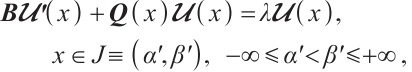

where 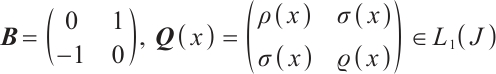 and
and  is real-valued Lebesgue measurable function on
  and
and  are
are  complex matrices such that rank
 and satisfy
  , where
  denotes the complex conjugate transpose of
  is the second order symplectic matrix. Besides, we are also interested in the spectral analysis of Dirac operator with the spectral parameter in boundary condition, which has a discrete spectrum consisting of an increasing infinite sequence of (real, simple) eigenvalues
  such that
  as
as  , see Ref. [11], and some remarkable works have been reached, see Refs. [12-13].
From the above literature, we notice that the research on problems (1)-(2) requires that the boundary conditions satisfy  Typically, the eigenparameter is only present in differential equations. Nonetheless, in numerous practical applications, including mechanics and acoustic scattering theory, it is necessary for the spectral parameter to be featured not only within the differential equations but also within the boundary conditions, see Ref. [14]. Recently, inverse spectral problems for Sturm-Liouville operators with non-self-adjoint eigenparameter-dependent boundary conditions have been studied via matrix representations and inverse matrix eigenvalue problems, see Ref. [15]. For the above model the condition
  may not be satisfied. Therefore, we hope to get the correlation spectrum properties of this kind of problems. For example, considering the self-adjointness of operators and the continuous dependence of eigenvalues, it is necessary to discuss the eigenvalue problem of a linear operator in a suitable Hilbert space. To address the limitation that these boundary conditions lack self-adjointness, we construct a suitable Banach space and an embedded mapping, and prove the continuity of the embedded mapping. Moreover, based on the definition of Fréchet derivative, we obtain the differentiability of eigenvalue bifurcation.
Our research plan is structured as follows. In Section 1, we introduce a self-adjoint operator eigenvalue problem and elucidate its critical spectral properties from various perspectives. In Section 2 and 3, leveraging the established continuity of the embedded mapping, we demonstrate the differentiability of the eigenvalue branch and present the corresponding derivative formulas.
1 Some Properties
This paper concerns eigenvalue problem of the form
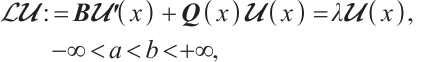

where  and every element in
  belongs to
 is the spectral parameter. Here, we require
  to satisfy
  and
and 
 are real numbers satisfying
 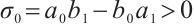 and
and 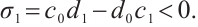
We first consider a linear operator eigenvalue problem derived from spectral problems (3)-(4). The inner product in the Hilbert space 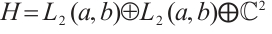 associated with

for  Define the operator
  acting in
  so that
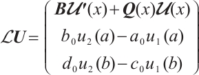
with the domain

Here  denotes the set of absolutely continuous and complex-valued functions on
  .
.
By immediate verification, we conclude that the problems (3)-(4) are equivalent to linear operator eigenvalue problem  . We now focus on discussing the properties of linear operator
  as follows.
Theorem 1
 is a self-adjoint operator in
  .
.
Proof In order to prove that the operator  is self-adjoint, we first need to prove that the domain of operator
  is dense in
  . Suppose
 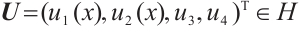 and
and  is orthogonal to
 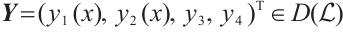 . We will prove
  . Since
  , for arbitrary
  , we have
 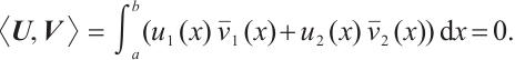 Since
Since  is dense in
  , we have
  , so
, so  . For any
  , through the inner product in
  , we get
  Since
Since  is arbitrary, we have
  Hence
Hence 
Secondly, we need to show that the operator  is symmetric. Let
  . For any
  , then

By the boundary condition (4), we have
Consequently, combining (5)-(7), we obtain
which implies that operator  is symmetric.
Since  is symmetric, it suffices to prove that for any
  and some
  satisfying
  , then
  and
and  , where
  . It means that
  satisfies following conditions:
(ⅰ) 
(ⅱ) 
(ⅲ) 
(ⅳ)  .
.
Indeed, the above conditions imply that 
Step 1 For arbitrary 
 , there is
  . Moreover, we arrive at
Namely,  . Since
  is symmetric, combined with
  , we can obtain
  . In view of the classical theory of differential operators, (ⅰ) and (ⅳ) hold.
Step 2 According (ⅳ) and the relation 
 , we have
In light of
Furthermore, one has

Using Naimark’s patching lemma[16], there exists a  such that

Then by (8), we have  . Similarly, we get

Moreover,  . Therefore, (ⅱ) holds. We can prove (ⅲ) by using the similar method, hence we omit the details. The proof is completed.
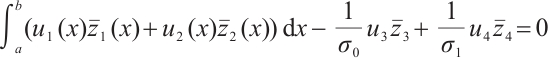
Corollary 1 The following assertions are true:
1) The two vector eigenfunctions corresponding to different eigenvalues of  and
and  are orthogonal in the following sense
2) All eigenvalues of the operator  are real, and all vector-eigenfunctions are real-valued.
Theorem 2[11] There exists an unboundedly decreasing sequence  of negative eigenvalues and an unboundedly increasing sequence
  of nonnegative eigenvalues of the boundary value problems (3)-(4):

Let 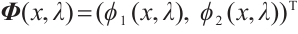 and
and 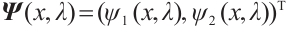 be the fundamental solutions of (3), which satisfy the initial condition

Then,  and
and  are linearly independent and entire functions of
  .
.
Denote
Lemma 1
 is an eigenvalue of (3)-(4) if and only if
  .
.
Proof By using similar methods in Ref. [10], we can obtain the assertion holds.
2 Continuous Dependence of Eigenvalues and Eigenfunction
Denote  . We introduce Banach space

equipped with the norm

For any  , where
  denotes the matrix normal. Let’s construct a boundary condition space
  ={
={ : the coefficient in (3)-(4), and
  hold}. Then
  is a closed subset of
  and inherits its topology
  .
.
Theorem 3 Let  , and
, and  be an eigenvalue of spectral problems (3)-(4). Then for any sufficiently small
  , there exists
  such that if
  , the spectral problems (3)-(4) have exactly one eigenvalue satisfying
Proof It is well known that  is eigenvalue of (3)-(4) if and only if Lemma 1 holds. It is obvious that
  is not constant with regard to λ since λ is isolated eigenvalue. Furthermore, for any
  is an entire function of
  . Hence, there exists
  such that
  for
for  . By the well known theorem on continuity of the roots of an equation as a function of parameters, see Ref. [17], the assertion holds.
The normalized eigenfunction  of spectral problems (3)-(4) is defined as follows:

Theorem 4 Let  is an eigenvalue of operator
  with
with  and
and  is a normalized eigenvector for
  . Then there exists a normalized eigenvector
  for
for  with
with  such that

as  both uniformly on
  .
.
Proof We know that  is simple. Let
  be a normalized eigenvector of operator
  . Then in view of inner product in the Hilbert space H, we have

and  is the corresponding eigenvalue. Theorem 3 means that there exists
  such that
  as
as  .
.
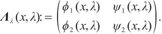
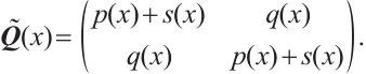
Denote the boundary conditions matrix as follows

Then  as
as  Besides, there exists
  satisfying the
  for
for  and
and  . Therefore, we obtain

as  both uniformly on
  . Let
. Let
Then the desired assertion holds. The proof is completed.
3 Differentiability of Eigenvalue
In this section, we will prove that the simple eigenvalue branch is differentiable for all parameters and obtain the differential expression for all parameter in the sense of Fréchet derivative.
Definition 1[17] A map  from an open set
  of the Banach space
  into the Banach space
  is Fréchet differentiable at a point
  if there exists a bounded linear operator
  such that in some neighborhood of the
  ,
,

Theorem 5 Let  be an eigenvalue for the operator
  for
for  and
and  be a normalized eigenvector of
  . Then
  is Fréchet differentiable with respect to all parameters in
  . Specifically, the derivative formulas of
  are given as follows:
Result 1 Fix all components of  except the boundary matrix
  and let
  denote the eigenvalue. Then
for all  , where
  .
.
Result 2 Fix all components of  except the boundary matrix
  and let
  denote the eigenvalue. Then
 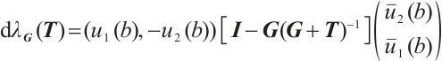 , for all
  , where
  .
.
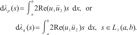
Result 3 Fix all components of  except
  or
or  and let
  denote the eigenvalue. Then
Result 4 Fix all components of  except
  , and let
  denote the eigenvalue. Then
such that  is symmetric and every element in
  belong to
  .
.
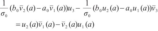
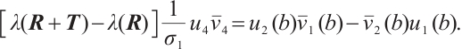
Proof 1) Let  denote the eigenvalue and corresponding normalize eigenvector. Direct computation yields

By (9)-(10) and integration by parts, we obtain

Let
By (4), we have

Using the similar method, we can obtain
Combining (11)-(13), we have

Let  , then the desired Result 1 can be obtained by Theorem 4.
2) Using the similar method, we can obtain Result 2.
3) Fix all components of  except
  (the situation for
  is similar). For
 denote eigenvalue and corresponding normalized eigenvector. Let
By (9) and (10), we have

By (4), we obtain 
Similarly, 
Hence

Then the desired Result 3 can be obtained.
4) In the same way, we can obtain Result 4. The proof is completed.
References
- Lott J. Eigenvalue bounds for the Dirac operator[J]. Pacific Journal of Mathematics, 1986, 125(1): 117-126. [Google Scholar]
- Levitan B M, Sargsjan I S. Sturm-Liouville and Dirac Operators[M]. Dordrecht: Kluwer Academic Publishers Group, 1991. [Google Scholar]
- Lunyov A A, Malamud M M. Stability of spectral characteristics of boundary value problems for 2×2 Dirac type systems. Applications to the damped string[J]. Journal of Differential Equations, 2022, 313: 633-742. [Google Scholar]
- Kh Amirov R, Keskin B, Ozkan A S. Direct and inverse problems for the Dirac operator with a spectral parameter linearly contained in a boundary condition[J]. Ukrainian Mathematical Journal, 2009, 61(9): 1365-1379. [Google Scholar]
- Du G F, Gao C H, Wang J J. Spectral analysis of discontinuous Sturm-Liouville operators with Herglotzs transmission[J]. Electronic Research Archive, 2023, 31(4): 2108-2119. [Google Scholar]
- Zhang M Z, Li K, Ju P J. Discontinuity of the nth eigenvalue for a vibrating beam equation[J]. Applied Mathematics Letters, 2024, 156: 109146. [Google Scholar]
- Lv X X, Ao J J, Zettl A. Dependence of eigenvalues of fourth-order differential equations with discontinuous boundary conditions on the problem[J]. Journal of Mathematical Analysis and Applications, 2017, 456(1): 671-685. [Google Scholar]
- Ao J J, Zhang L. An inverse spectral problem of Sturm-Liouville problems with transmission conditions[J]. Mediterranean Journal of Mathematics, 2020, 17(5):1-24. [Google Scholar]
- Zhang M Z, Li K. Dependence of eigenvalues of Sturm-Liouville problems with eigenparameter dependent boundary conditions[J]. Applied Mathematics and Computation, 2020, 378: 125214. [Google Scholar]
- Li K, Zhang M Z, Zheng Z W. Dependence of eigenvalues of Dirac system on the parameters[J]. Studies in Applied Mathematics, 2023, 150(4): 1201-1216. [Google Scholar]
- Kerimov N B. A boundary value problem for the Dirac system with a spectral parameter in the boundary conditions[J]. Differential Equations, 2002, 38(2): 164-174. [Google Scholar]
- Allahverdiev B P. A nonself-adjoint 1D singular Hamiltonian system with an eigenparameter in the boundary condition[J]. Potential Analysis, 2013, 38(4): 1031-1045. [Google Scholar]
- Allahverdiev B P. Extensions, dilations and functional models of Dirac operators[J]. Integral Equations and Operator Theory, 2005, 51(4): 459-475. [Google Scholar]
- Binding P A, Browne P J, Watson B A. Equivalence of inverse Sturm-Liouville problems with boundary conditions rationally dependent on the eigenparameter[J]. Journal of Mathematical Analysis and Applications, 2004, 291(1): 246-261. [Google Scholar]
- Zhang L, Ao J J, Lü W Y. Inverse Sturm-Liouville problems with a class of non-self-adjoint boundary conditions containing the spectral parameter[J]. Wuhan University Journal of Natural Sciences, 2024, 29(6): 508-516. [Google Scholar]
- Naimark M A. Linear Differential Operator[M]. New York: Frederick Ungar Publishing Company, 1968. [Google Scholar]
- Zettl A. Sturm-Liouville Theory[M]. Providence RI: American Mathematical Society, 2005. [Google Scholar]
Current usage metrics show cumulative count of Article Views (full-text article views including HTML views, PDF and ePub downloads, according to the available data) and Abstracts Views on Vision4Press platform.
Data correspond to usage on the plateform after 2015. The current usage metrics is available 48-96 hours after online publication and is updated daily on week days.
Initial download of the metrics may take a while.