| Issue |
Wuhan Univ. J. Nat. Sci.
Volume 30, Number 3, June 2025
|
|
|---|---|---|
| Page(s) | 241 - 252 | |
| DOI | https://doi.org/10.1051/wujns/2025303241 | |
| Published online | 16 July 2025 | |
Mathematics
CLC number: O175
∑-Shaped Connected Component of Positive Solutions for One- Dimensional Prescribed Mean Curvature Equation in Minkowski Space
Minkowski 空间中一维给定平均曲率方程正解的∑-型连通分支
College of Mathematics and Statistics, Northwest Normal University, Lanzhou 730070, Gansu, China
† Corresponding author. E-mail: This email address is being protected from spambots. You need JavaScript enabled to view it.
Received:
5
December
2024
Abstract
In this work, we demonstrate that the existence of an ∑-shaped connected component within the set of positive solutions for the one-dimensional prescribed mean curvature equation in Minkowski space 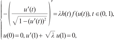 with boundary conditions having parameter in two cases
  and
and  by using upper and lower solution method, where
  is a parameter,
  is monotonically increasing and
  ,
,  is a nonincreasing function and
  .
.
摘要
运用上下解方法证明 Minkowski 空间中一维给定平均曲率方程 
 在 和
在 和  两种情形下正解集
 型连通分支的存在性,其中,
 为参数,
为参数, 单调递增且满足
  ,
, 是单调递减函数且
  .
.
Key words: boundary conditions with parameters / positive solutions / the upper and lower solution method / asymptotic property
关键字 : 边界条件带参数 / 正解 / 上下解定理 / 渐进性质
Cite this article: QI Tiaoyan, LU Yanqiong. ∑-Shaped Connected Component of Positive Solutions for One- Dimensional Prescribed Mean Curvature Equation in Minkowski Space[J]. Wuhan Univ J of Nat Sci, 2025, 30(3): 241-252.
Biography: QI Tiaoyan, female, Master candidate, research direction: difference equations and their applications. E-mail: This email address is being protected from spambots. You need JavaScript enabled to view it.
Foundation item: Supported by the National Natural Science Foundation of China (12361040)
© Wuhan University 2025
 This is an Open Access article distributed under the terms of the Creative Commons Attribution License (https://creativecommons.org/licenses/by/4.0), which permits unrestricted use, distribution, and reproduction in any medium, provided the original work is properly cited.
0 Introduction
The boundary value problem in which the boundary conditions involve parameters is one of the most significant problems in the mathematical theory. In 1994, Binding was the first to propose the Sturm Liouville problems with boundary conditions dependent on eigenparameters[1]. In 1999, Hai[2] used the prior estimation method to prove the existence of solutions for boundary value problem
with boundray conditions having parameters. Since then, many different problems with parameters under boundary conditions have been studied respectively by Marinets et al[3], and a great deal of fruitful results have been achieved, which can be found in Refs. [4-7]. Fonseka et al[6-7] investigated the positive solution of the boundary value problem with two boundary conditions having parameters by employing the upper and lower solution method. They proved the existence and multiplicity of the positive solutions and obtained the bifurcation diagram of the above positive solutions by using the time mapping method. Particularly, Fonseka et al[6] discussed the existence and multiplicity results of the steady-state reaction diffusion equation
via the upper and lower solution method in three cases of  ,
,  and
and  . Further, they established a unique result for
  and
and  . In the above equation,
  is a parameter,
  is an increasing function which is sublinear at infinity,
 is a nonin-creasing function with
  and there exist constants
  ,
,  such that
  for all
  , and
, and  is an increasing function such that
  .
.
The prescribed mean curvature equation addressed in this paper is regarded as a significant problem in partial differential equations and possesses extensive applications in other domains like physics and biology, such as the shape of the human cornea[8-9], drops of capillary droopiness[10], micro electronic mechanical systems, and corresponding models of large spatial gradients[11]. Specifically, the Dirichlet problem with the Minkowski-curvature operator
has drawn the attention of numerous scholars. Especially, the existence and multiplicity of positive solutions for the Dirichlet problem with the one-dimensional Minkowski-curvature operator
have been extensively studied by employing the variational method, the upper and lower solution method, and the time mapping method. See Refs. [12-20], where  is parameter,
  and
and  . It is obvious that the problems in the above references merely study the positive solutions of the Dirichlet problem with the mean curvature operator in Minkowski space in the case where the nonlinear term has a parameter. However, the prescribed mean curvature boundary value problem where both the nonlinear term and the boundary conditions have parameters must be further considered to accurately describe the corresponding physical phenomena.
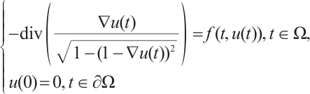
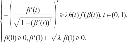
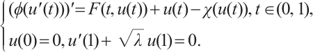
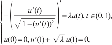
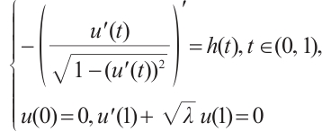
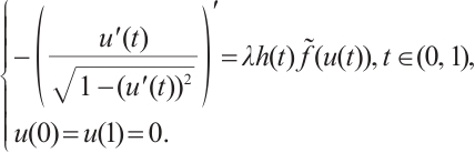
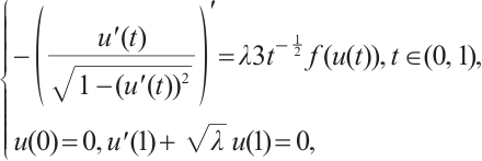
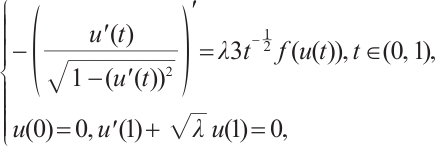
Inspired by the above-mentioned papers, we explore the existence and multiplicity of positive solutions for the one-dimensional prescribed mean curvature problem in Minkowski space
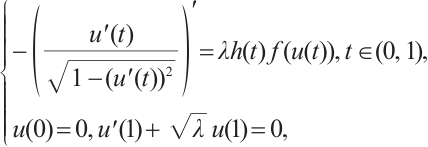 (1)
(1)
with boundary conditions having parameter in two cases  and
and  by using upper and lower solution method, where
  is a parameter,
  is monotonically increasing and
 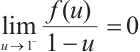 ,
,
 is a nonincreasing function and
  .
.
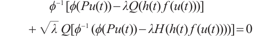
From the conclusion of Ref. [15], it follows that problem (1) has a positive solution  if and only if the problem
 (2)
(2)
has a positive solution, and  ,
,  .
.
Let  is monotone increasing homeomorphism defined by
  , then
  and
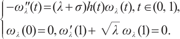
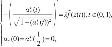
and  is also monotone increasing homeomorphism and bounded. Let us consider the eigenvalue problem
 (3)
(3)
Based on the results of Ref. [6], the problem (3) has principal eigenvalue  , and the eigencurve
  is Lipschitz continuous, strictly decreasing and convex. Further
  , where
  is the principal eigenvalue of
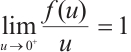
Throughout the paper we will assume that  satisfies:
 ;
; 
 for some
  .
.
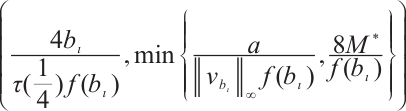
Let 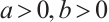 and
and  . Define
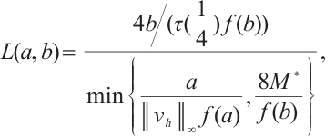
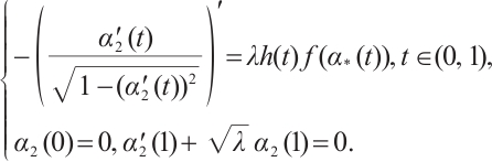
where  is the solution of the problem
 (4)
(4)
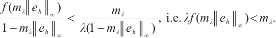
First, we state the main results for the case:  .
.
Theorem 1 Assume  and
and  hold. Then problem (1) has no positive solution for
  and has at least one positive solution for
  . Further, if there exist
  such that

 and
and  . Then problem (1) has at least three positive solutions for
  .
.
Theorem 2 Assume  ,
, and
and  hold. Then problem (1) has least one positive solution
  for
for  such that
  .
.
Next, we state the main results for case:  .
.
Theorem 3 Assume  . Then problem (1) as at least one positive solution for
  . Further, if there exist
  ,
,  and
and  such that
  ,
,  and
and  . Then (1) has at least three positive solutions for
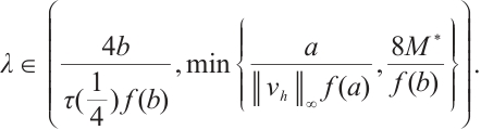
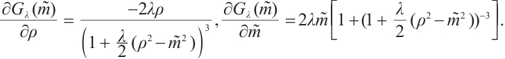
Note that the connected component of positive solutions of (1) is the  shaped under the assumptions of Theorem 1 or Theorem 3. Figure 1(a) illustrated the main results of Theorem 1, Fig.1 (b) illustrated the main results of Theorem 3. The rest of the paper is organized as follows. In Section 1, we introduce some lemmas needed to prove the main theorems. In Section 2, we use the time-mapping method to prove that problem
  has at least one positive solution when
  , which will help to construct the subsolution of
  . In Section 3, we give proofs of the main results. In Section 4, we show some examples.
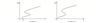 |
Fig. 1 Bifurcation diagram for problem (1) |
1 Preliminaries
Let  , it is not hard to verify that
  endowed with the norm
 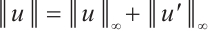 is Banach space.
We donote by  , and the continuous projects defined by
 ,
,  and define the continuous linear operator
  ,
,  ,
,  . Integration of both sides of the equation in problem (1) from
  to
to  implies that
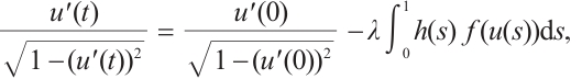
i.e.
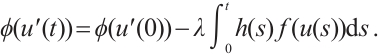
Applying  to the above equation, we get that
 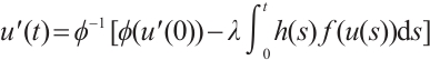 . Furthermore, we integrate the above equation from
  to
to  , it follows that
 (5)
(5)
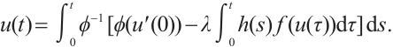
Combining  , we obtain that
  satisfies
 (6)
(6)
which yields that
 (7)
(7)
Lemma 1 For  , there is a unique
  such that
 and
and  is continuous.
Proof For any given  , define the function
  as follows:
There are  such that
then there exists  such that
  .
.
Next we prove uniqueness of  . Let
. Let  such that
  , hence there exists
  such that
Since  and
and  is bijection,
  . Finally, from the continuity of
  ,
,  and
and  , we can conclude that
  is continuous.
Lemma 2
 being a solution to problem (1) is equivalent to
  being a fixed point of

Proof It follows from Lemma 1 that there exists a unique  such that (7) holds, so the operator equation of problem (1) is
  . It is obvious that
  , hence its inverse mapping
  is a bounded operator, and it follows from (5) that
  .
.
Next, we introduce definitions of a (strict) subsolution and a (strict) supersolution of problem (1) and establish the upper and lower solution theorem that is used to prove existence and multiplicity results of (1).
By a supersolution of the problem (1) we define  that satisfies
 (8)
(8)
By a supersolution of the problem (1), we define 
 that satisfies
 (9)
(9)
By a strict subsolution (supersolution) of (1) we mean a subsolution (supersolution) which is not a solution of (1).
Lemma 3 Let  and
and  such that
  . If
. If
 (10)
(10)
and  ,
,  , then
  .
.
Proof Suppose on the contrary that there exists  such that
  , then
  , and there exists a sequence
  on
on  such that
  . The fact that
  is monotone increasing homeomorphism implies that
  .
.
By the definition of the derivative we get that
 (11)
(11)
This together with (10) and (11) concludes that  , which is contradictory. Therefore,
  for all
  .
.
Corollary 1 Let  such that
 .If
.If  for any
  , then
  .
.
Lemma 4 Let  and
and  be a subsolution and a supersolution of (1), respectively, such that
  , then (1) has a solution
  such that
  .
.
Proof Let  be the continuous function which is defined by
and define  by
by  . Obviously,
  is continuous and bounded.
Next we consider the auxiliary problem
 (12)
(12)
First, the problem (12) has at least one solution  by the Schauder fixed theorem. Next, we only show that
  ,
,  , so
, so  is a solution of (1).
Suppose on the contrary that there exists  such that
  >0. Because
  , there exist two sequence
  and
and  such that
  and
and  . Without loss of generality, it follows from
  that
that  . By
. By  is an increasing homeomorphism, we get that
  .
.


Moreover,  is a subsolution of (1), it yields that
This is a contradiction, thus  . In addition, by the similar arguments, it follows that
  . Therefore
  is a solution of problem (1).
Lemma 5 Let  and
and  be a subsolution and supersolution of (1) respectively such that
  . Let
. Let  and
and  be a strict subsoltion and a strict supersolution of (1) respectively satisfying
  and
and  . Then (1) has at least three solutions
  ,
,  and
and  , where
  ,
,  and
and  .
.
Proof Let  denote the the unique positive solution of
Let  ,
,  ,
,  ,
,  . It is not difficult to verify that
  endowed with the norm
  is Banach space, then
  ,
,  and
and  are non-empty closed convex subsets of Banach space
  . In the following, we will prove that
  is completely continuous and strongly increasing.
In fact,  and
and  are disjoint subsets of
  . The map
  is restricted to
  . Since
  is increasing and
  ,
,  are subsolution and supersolution of (1) respectively (
 ), we have that
  , i.e.
  . Similarly,
  . Since
  is a strict supersolution of (2), we have that
  . By Ref. [21], Corollary 6.2,
  has a maximal fixed point in
  and
and  . Similarly,
  has a minimal fixed point in
  and
and  , because
  is a strict subsoluton of (1).
Notice that

it follows from Lemma 3 that  , hence there exists a constant
  such that
  . Similarly there exists a constant
  such that
  . Define

then  is open set,
  . Hence
  has non-empty interior. Let
  be the largest open set in
  , which contain
  such that
  has no fixed point in
  . Finally by Ref. [22], Lemma 3.8,
  has a third fixed point
  . Therefore, problem (1) has at least three solutions
  ,
,  and
and  .
.
2 The Autonomous Case of  ,
, 
We consider the quasilinear problem
 (13)
(13)
where  is a parameter.
Multiplying the differential equation in (13) by  and integrating from
  to
to  , we get that
  , where
  . From Ref. [8], Lemma 2.3, there exists
  such that
  . Now we choose
  in (13) and yield
 (14)
(14)
 (15)
(15)
Let  , further integration from
  to
to  for (14) and integration from
  to
to  for (15), it follows that
 (16)
(16)
 (17)
(17)
We obtain by combining (16) and (17) that
 (18)
(18)
Finally, from boundary value  and (15), we can get
 (19)
(19)
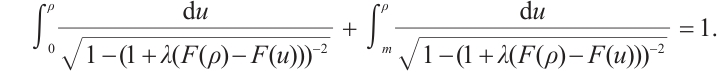
Let  be a fixed value and
  . By (19), it is easy to compute that
 (20)
(20)
further 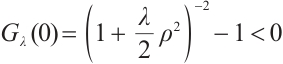 ,
,  , so it follows from the intermediate value theorem that there exists
  such that (19) holds.
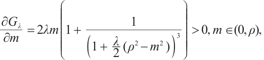
Lemma 6 For any fixed  ,
,  for
for  .
.
Proof By (19), we get that  . It is easy to compute that
Thus  , i.e.
  .
.
Definition 1 For any given  , we define a map
 (21)
(21)
called the time map of problem (13).
In fact, the existence of a solution to problem (13) is equivalent to the existence of a solution to  , see Refs. [19, 23].
Theorem 4 For any given  , there exists
  satisfying (18) and (19) such that problem (13) has at least one positive solution for any
  .
.
Proof Clearly, for any fixed  , there exists
  such that
  . Now, let
  in (21), we show that
 (22)
(22)
It is easy to compute that 
 , and
, and 

Therefore, there exist  and
and  , such that
  holds. Then problem (13) has at least one positive solution.
Finally, we discuss the range of value of  when a positive solution exists for problem (13). The fact together with (18) concludes that
Therefore,  .
.
Next, we show that  . From the definition of
  , we get that
  . Hence, there exists
  for any
  such that
  ,
,  and it follows that
This together with (18) implies that
Therefore, we yield that for  small enough as
  ,
,  , i.e.
  .
.
In consequence, the problem (13) has at least one positive solution for any  .
.
Remark 1 In the case of  ,
,  , the principal eigenvalue of problem
has eigenvalue  , and the corresponding eigenfunction is
  ,
,  .
.
3 The Proof of Main Results
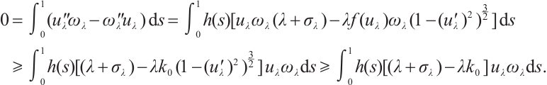
Proof of Theorem 1 We first show the nonexistence for  . Let
. Let  be the principal eigenvalue and
  be the corresponding normalized eigenfunction of
We note that  for
for  and
and  for
for  , the detail see Ref. [24]. Supppose on the contrary that
  be a positive solution of (1) for
  . Note that there exists
  such that
  for
for  , and
, and
 (23)
(23)
Clearly, it is easy to see that  for
for  . Thus there exists constant
  (independent of
  ) such that
  . Besides, by (23), it follows that
  , i.e.
  . This is a contradiction, hence (1) has no positive solution for
  .
.
Next, we show that the existence of positive solution of (1) for  . Let
. Let  , where
  is solution of
and  . Then
  and
and  .
.
Since  , for all
  , there exists
  such that
  ,
,  . Furthermore, choosing
  , we have that
 (24)
(24)
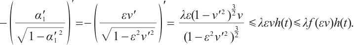
Next, we prove that  is an upper solution to problem (1). By
  and (24), we conclude that

In addition, we get that  and
and  , thus
  is a supersolution.
Let  with
with  , where
  is positive solution of (13) according to Theorem 4. Since
  ,
,  . Therefore, for any
  , there exists
  such that
 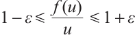 . Hence, for
  , we have that
Obviously  and
and  , thus
  is a subsolution of (2). Now choosing
  to ensure that
  . By Lemma 1 there exists a positive solution
  for
for  .
.
Finally, we establish the multiplicity result of positive solution of (1). Let  such that
  is strictly increasing on
  . We first construct a strict subsolution of the Dirichlet problem
 (25)
(25)
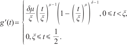
Define  satisfying
where  is defined such that the function
  is strictly increasing on
  and
and  . For
. For  , let
, let
and  ,
,  , where
  . By computing, we get that
Assume that there exists a constant  such that
  , and define
  . Since
  ,
,  . Define
  on
on  to be the solution of
 (26)
(26)
and extend  on
on  such that
  , where
  has a maximum value at
  and is symmetric about
  , see Ref. [17].
Claim
 ,
,  .
.
Based on the claim, it follows that

Since  ,
,  . Therefore,
  is a strict subsolution. Now, we prove the claim is true. First, we show that
  ,
,  .
.
Define  , then
  . Recall that (26). Integration from
  to
to  with
with  and noting that
  , we obtain that
 (27)
(27)
Now we choose  . Since
  , we can choose
  such that
  . Hence for all
  ,
, . Clearly,
  ,
,  for all
  . We obtain that

Since  , we have
  for all
  . By symmetry of the solution of (26),
  for all
  .
.
Next, we show that  Recall that
  ,
,  . Integrating from
  to
to  , we have
Furthermore, 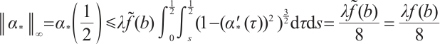 . This together with
  yields
  . Hence
  for
for  . Moreover
  is a strict subsolution of problem (1).
Let  be the first interation of
  , then
  be the soluton to the problem
Then 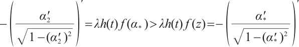 . By Corollary 1, we have that
  . Hence, it is not difficult to verfy that
  is a strict subsolution of (1).
Finally, we construct a strict supersolution for  , where
  is a constant. Let
  , where
  is defined by (4). Then

On the other hand,  satisifies
  and
and  . Therefore
  is a strict supersolution for
  . Further, we can choose
  and
and  such that
  and
and  . Since
  ,
,  . Therefore (1) has at least three positive solutions from Lemma 5.
Proof of Theorem 2 By  , there exists
  such that
  for
for  . Let
. Let  , where
  . It follows that
  and
and  from
from  ,
,  and
and  . By the Taylor's series
  ,
, , it concludes that
Therefore,  is a supersolution of (1) for
  and
and  . Let
. Let  be as in the proof of Theorem 1. Choosing
  , we can note that
  . By Lemma 2, there exists a positive solution
  for
for  and
and  such that
  .
.
Proof of Theorem 3 First of all, we show the existence of positive solution for  . Clearly,
  is a strict subsoluion of (1). Let
 be as in the proof of Theorem 1, then is a supersolution of (1). Further, by Lemma 1, there exists
  . Next, the proof of multiplicity is similar to that of Theorem 1, we omit it.
4 Examples
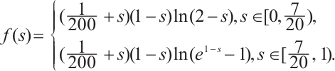
Example 1 Let us consider the following problem
 (28)
(28)
where
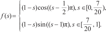
It is obvious that  . Moreover, we note that
  satisfies
  ,
,  and
and  . Let
. Let  , then
  . Let
. Let  and
and  , then we can choose
  such that
  . Let
. Let  be as in (4). It is easy to compute that
  ,
,  . Then we obtain that
  . Hence
  <1. Next, let
  . Then
  . Therefore, problem (28) has at least three positive solutions for
 by Theorem 1.
Example 2 Let us consider the following problem
 (29)
(29)
where
It is obvious that  . Moreover, we note that
  satisfies
  ,
,  and
and 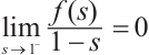 . The following is similar to Example 1, so we omit it.
References
- Binding P A, Browne P J, Seddighi K. Sturm-Liouville problems with eigenparameter dependent boundary conditions[J]. Proceedings of the Edinburgh Mathematical Society, 1994, 37(1): 57-72. [Google Scholar]
- Hai D D. Positive solutions for semilinear elliptic equations in annular domains[J]. Nonl Anal: Theo, Meth & Appl, 1999, 37(9): 1051-1058. [Google Scholar]
- Marinets V V, Pitovka O Y. On a problem with a parameter in the boundary conditions[J]. Nauk Visn Uzhgorod Univ Ser Mat Inform, 2005 (10-11): 70-76. [Google Scholar]
- Li Z L. Second-order singular nonlinear boundary value problem with parameters in the boundary conditions[J]. Adv Math, 2008, 37(3): 353-360(Ch). [Google Scholar]
- Aslanova N, Bayramoglu M, Aslanov K. On one class eigenvalue problem with eigenvalue parameter in the boundary condition at one end-point[J]. Filomat, 2018, 32(19): 6667-6674. [Google Scholar]
- Fonseka N, Muthunayake A, Shivaji R, et al. Singular reaction diffusion equations where a parameter influences the reaction term and the boundary conditions[J]. Topological Methods in Nonlinear Analysis, 2021, 57(1): 221-242. [Google Scholar]
- Acharya A, Fonseka N, Quiroa J, et al. σ-shaped bifurcation curves[J]. Adv in Nonl Anal, 2021, 10(1): 1255-1266. [Google Scholar]
- Hai D D. Positive solutions to a class of elliptic boundary value problems[J]. J of Math Anal and Appl, 1998, 227(1): 195-199. [Google Scholar]
- Njoku F I, Omari P, Zanolin F. Multiplicity of positive radial solutions of a quasilinear elliptic problem in a ball[J]. Adv in Diff Equ, 2000, 5(10-12): 1545-1570. [Google Scholar]
- Bereanu C, Jebelean P, Mawhin J. Radial solutions for Neumann problems involving mean curvature operators in Euclidean and Minkowski spaces[J]. Mathematische Nachrichten, 2010, 283(3): 379-391. [Google Scholar]
- Jean M. Radial solutions of Neumann problem for periodic perturbations of the mean extrinsic curvature operator[J]. Milan Journal of Mathematics, 2011, 79(1): 95-112. [Google Scholar]
- Bartnik R, Simon L. Spacelike hypersurfaces with prescribed boundary values and mean curvature[J]. Communications in Mathematical Physics, 1982, 87(1): 131-152. [Google Scholar]
- Azzollini A. On a prescribed mean curvature equation in Lorentz-Minkowski space[J]. Journal de Mathématiques Pures et Appliquées, 2016, 106(6): 1122-1140. [Google Scholar]
- Born M, Infeld L. Foundations of the new field theory[J]. Nature, 1933, 132(3348): 1004. [Google Scholar]
-
Bereanu C, Mawhin J. Existence and multiplicity results for some nonlinear problems with singular
 -Laplacian[J]. J of Diff Equ, 2007, 243(2): 536-557.
[Google Scholar]
-Laplacian[J]. J of Diff Equ, 2007, 243(2): 536-557.
[Google Scholar]
- Anuradha V, Shivaji R. A quadrature method for classes of multi-parameter two point boundary value problems[J]. Applicable Analysis, 1994, 54(3-4): 263-281. [Google Scholar]
- Ma R Y, Lu Y Q. Multiplicity of positive solutions for second order nonlinear dirichlet problem with one-dimension Minkowski-curvature operator[J]. Adv Nonl Studies, 2015, 15(4): 789-803. [Google Scholar]
- Dai G W. Bifurcation and positive solutions for problem with mean curvature operator in Minkowski space[J]. Cal of Vari and Part Diff Equ, 2016, 55(4): 72. [Google Scholar]
- Xu M, Ma R Y. S-shaped connected component of radial positive solutions for a prescribed mean curvature problem in an annular domain[J]. Open Mathematics, 2008, 17: 929-941. [Google Scholar]
- Lu Y Q, Li Z Q, Chen T L. Multiplicity of solutions for non-homogeneous dirichlet problem with one-dimension minkowski-curvature operator[J]. Qualitative Theory of Dynamical Systems, 2022, 21(4): 145. [Google Scholar]
- Amann H. Fixed point equations and nonlinear eigenvalue problems in ordered Banach spaces[J]. SIAM Review, 1976, 18(4): 620-709. [Google Scholar]
- Dhanya R, Ko E, Shivaji R. A three solution theorem for singular nonlinear elliptic boundary value problems[J]. J of Math Anal and Appl, 2015, 424(1): 598-612. [Google Scholar]
- Gao H L, Xu J. Bifurcation curves and exact multiplicity of positive solutions for Dirichlet problems with the Minkowski-curvature equation[J]. Boundary Value Problems, 2021, 2021: 81. [Google Scholar]
- Goddard II J, Morris Q A, Robinson S B, et al. An exact bifurcation diagram for a reaction-diffusion equation arising in population dynamics[J]. Boundary Value Problems, 2018, 2018(1): 170. [Google Scholar]
All Figures
|
Fig. 1 Bifurcation diagram for problem (1) |
| In the text | |
Current usage metrics show cumulative count of Article Views (full-text article views including HTML views, PDF and ePub downloads, according to the available data) and Abstracts Views on Vision4Press platform.
Data correspond to usage on the plateform after 2015. The current usage metrics is available 48-96 hours after online publication and is updated daily on week days.
Initial download of the metrics may take a while.