| Issue |
Wuhan Univ. J. Nat. Sci.
Volume 30, Number 3, June 2025
|
|
|---|---|---|
| Page(s) | 235 - 240 | |
| DOI | https://doi.org/10.1051/wujns/2025303235 | |
| Published online | 16 July 2025 | |
Mathematics
CLC number: O175
Liouville Theorem for 3D Steady Q-Tensor System of Liquid Crystal in Mixed Lorentz Spaces
三维稳态Q-tensor液晶流系统在混合Lorentz空间中的Liouville型定理
1 College of Science, China Three Gorges University, Yichang 443002, Huibei, China
2 Three Gorges Mathematical Research Center, China Three Gorges University, Yichang 443002, Huibei, China
† Corresponding author. E-mail: This email address is being protected from spambots. You need JavaScript enabled to view it.
Received:
25
June
2024
Abstract
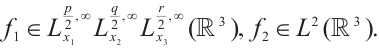
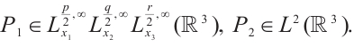
In this paper, we study Liouville theorem for 3D steady  -tensor system of liquid crystal in mixed Lorentz spaces. We obtain
  on the conditions that
 and
and  which extends some known results.
摘要
本文在混合Lorentz空间中研究了三维稳态 -tensor液晶系统的Liouville定理。我们在条件
 和
和  下得到
下得到  这一结论,它推广了一些已有的结果。
Key words: mixed Lorentz spaces / Q-tensor system of liquid crystal / Liouville theorem
关键字 : 混合Lorentz空间 / Q-tensor液晶流系统 / Liouville定理
Cite this article: WAN Mengru, DENG Xuemei, BIE Qunyi. Liouville Theorem for 3D Steady Q-Tensor System of Liquid Crystal in Mixed Lorentz Spaces[J]. Wuhan Univ J of Nat Sci, 2025, 30(3): 235-240.
Biography: WAN Mengru, female, Master candidate, research direction: partial differential equations. E-mail: This email address is being protected from spambots. You need JavaScript enabled to view it.
Foundation item: Supported by the National Natural Science Foundation of China (11871305)
© Wuhan University 2025
 This is an Open Access article distributed under the terms of the Creative Commons Attribution License (https://creativecommons.org/licenses/by/4.0), which permits unrestricted use, distribution, and reproduction in any medium, provided the original work is properly cited.
0 Introduction
In this paper, we study the following 3D stationary  -tensor system of liquid crystal:
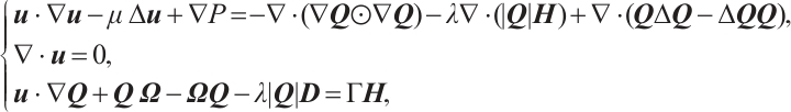 (1)
(1)
with
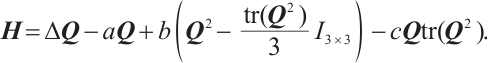
Here 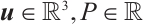 and
and

stand for the flow velocity, the scalar pressure and the nematic tensor order parameter, respectively. The parameters 
 and
and  represent the viscosity coefficient, the rotational viscosity and the nematic alignment, respectively. The coefficients
 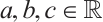 with
with  are constants.
  is the symmetric additional stress tensor.
  , and
, and  are the symmetric and skew symmetric, respectively, where the notation
  represents the transposition of a matrix.
When  , system (1) reduces to the 3D stationary Navier-Stokes system
 (2)
(2)
For system (2), a well-known result on the Liouville theorem is given by Galdi[1], which concludes if  then
then  . Chae-Wölf[2] gave the following logarithmic improvement
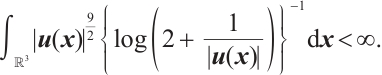
Kozono-Terasawa-Wakasugi[3] extended Galdi's result[1] to the Lorentz spaces  . Luo and Yin[4] showed that if the solution to system (2) satisfies
 (3)
(3)
then  , where
For more Liouville theorem results of system (2), one could refer to Refs. [5-9] and references therein.
In recent years, the  -tensor system of liquid crystal (1) has received much attention. However, there are few results on its Liouville theorem. Gong et al[10] proved that if

then  . Later, Lai and Wu[11] generalized the conditions to
 (4)
(4)
On Liouville theorem for many other models, there are also numerous results (see for example Refs. [12-15]).
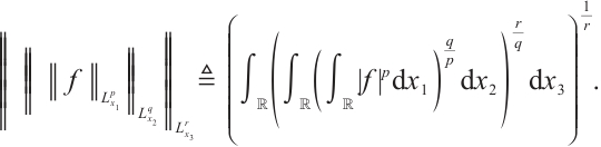
Inspired by the works mentioned above in this paper, we will prove that there is only the trivial solution for the steady  -tensor system of liquid crystal model in mixed Lorentz spaces. First of all, we recall the definition of mixed Lorentz spaces.
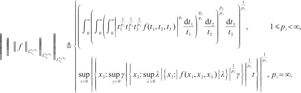
Definition 1 Assume the indexes  and
and  satisfying
  ,
,  , or
, or  . A mixed Lorentz space
  is the set of functions for which the following norm is finite:
The main result of the paper is stated in the following theorem.
Theorem 1 Let  be a smooth solution to system (1) in
  . If
. If

then  .
.
Remark 1 In the case of  in Theorem 1, the sufficient condition coincides with (4) obtained in previous work[11]. In addition, due to the following embedding (see for example Ref. [16])
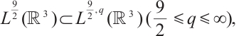 (5)
(5)
we deduce that our result extends Gong et al 's result in Ref. [10].
When  , we obtain the following Liouville theorem for the Navier-Stokes equations (2), which is a supplement to the result of Ref. [4] (see (2)).
Corollary 1 Let 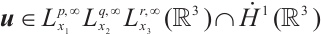 be a smooth solution to the Navier-Stokes equations (2) in
  . If
. If 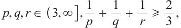 then
then  .
.
1 Proof of Theorem 1
In this section, we give the proof of Theorem 1. To streamline the presentation, set

We firstly recall the following lemma.
Lemma 1[17] Let  then
then  .
.
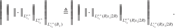
Proof We consider a smooth cut-off function  such that

For each  , defining
then, one has
Moreover, there is a constant  independent of
  such that
  for
for 
Multiplying the first equation and the second equation of (1) by  and
and 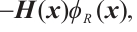 respectively, we know
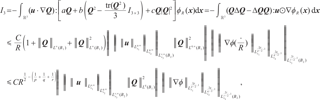
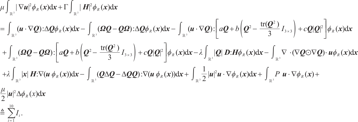 (6)
(6)
Firstly, since  is symmetric and
  is skew symmetric, we deduce
  . For
. For  and
and  , using Hölder inequality, we obtain
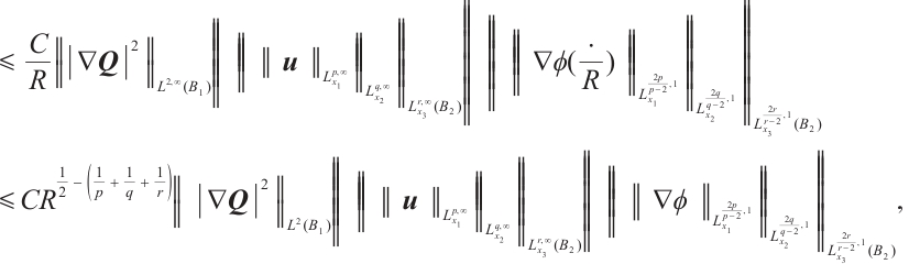 (7)
(7)
 (8)
(8)
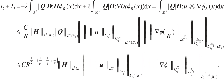 (9)
(9)
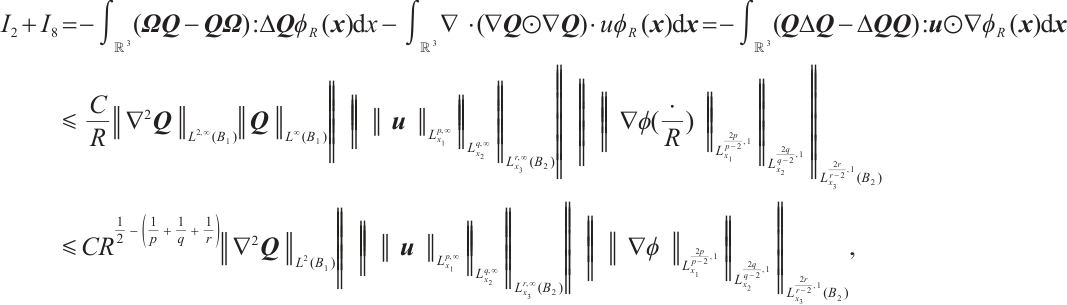
For  and
and  , along the same line, we have
 (10)
(10)
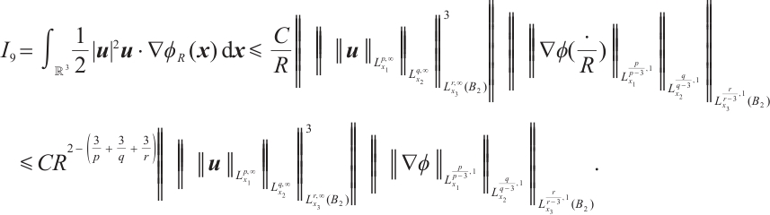 (11)
(11)
For  , note that

Let 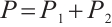 such that
  and
and 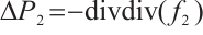 , where

In view of the conditions 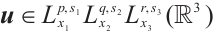 and
and  , we obtain that
By Calderron-Zygmund theorem, it follows that
Then,
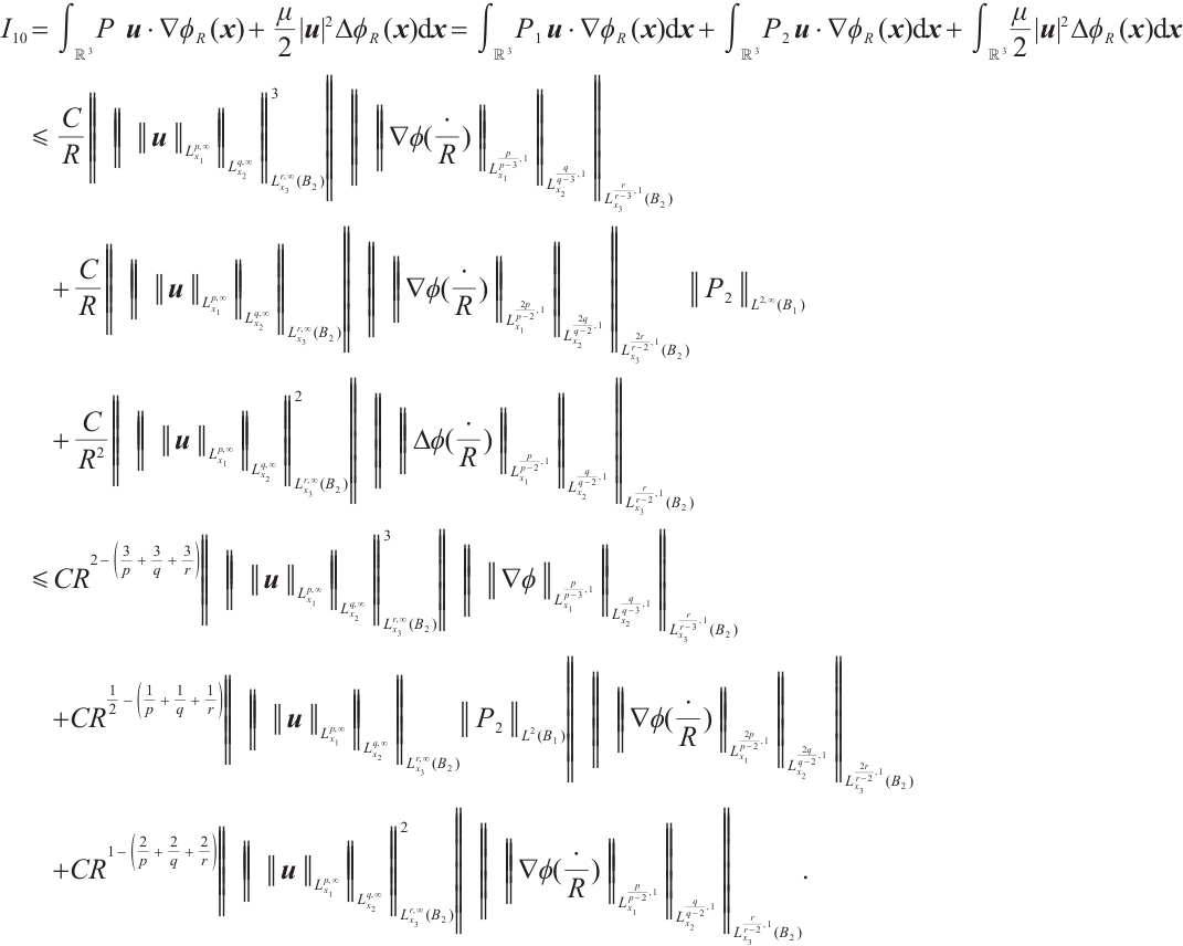 (12)
(12)
Therefore, when  , we can obtain
 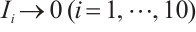 . Thanks to the Sobolev embedding, we have

then  and
and  . By the definition of
  , we observe
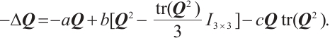 (13)
(13)
Taking the inner product of the equation (13) with  , and by Lemma 1, one yields
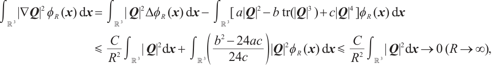
which combined with 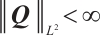 , concludes
  . The proof of Theorem 1 is completed.
References
- Galdi G P. An Introduction to the Mathematical Theory of the Navier-Stokes Equations: Steady-State Problems[M]. Second Edition. New York: Springer-Verlag, 2011. [Google Scholar]
-
Chae D, Wolf J. On Liouville type theorems for the steady Navier-Stokes equations in
 [J]. Journal of Differential Equations, 2016, 261(10): 5541-5560.
[Google Scholar]
[J]. Journal of Differential Equations, 2016, 261(10): 5541-5560.
[Google Scholar]
- Kozono H, Terasawa Y, Wakasugi Y. A remark on Liouville-type theorems for the stationary Navier-Stokes equations in three space dimensions[J]. Journal of Functional Analysis, 2017, 272(2): 804-818. [Google Scholar]
- Luo W, Yin Z Y. The Liouville theorem and the L2 decay for the FENE dumbbell model of polymeric flows[J]. Archive for Rational Mechanics and Analysis, 2017, 224(1): 209-231. [Google Scholar]
- Chae D. Liouville-type theorems for the forced Euler equations and the Navier-Stokes equations[J]. Communications in Mathematical Physics, 2014, 326(1): 37-48. [Google Scholar]
- Chae D, Yoneda T. On the Liouville theorem for the stationary Navier-Stokes equations in a critical space[J]. Journal of Mathematical Analysis and Applications, 2013, 405(2): 706-710. [Google Scholar]
- Superiore S, Gilbarg D, Weinberger H, et al. Asymptotic properties of steady plane solutions of the Navier-Stokes equations with bounded Dirichlet integral[J]. Annali Della Scuola Normale Superiore Di Pisa-classe Di Scienze, 1978, 5: 381-404. [Google Scholar]
- Koch G, Nadirashvili N, Seregin G A, et al. Liouville theorems for the Navier-Stokes equations and applications[J]. Acta Mathematica, 2009, 203(1): 83-105. [Google Scholar]
- Korobkov M, Pileckas K, Russo R. The Liouville theorem for the steady-state Navier-Stokes problem for axially symmetric 3D solutions in absence of swirl[J]. Journal of Mathematical Fluid Mechanics, 2015, 17(2): 287-293. [Google Scholar]
- Gong H J, Liu X G, Zhang X T. Liouville theorem for the steady-state solutions of Q-tensor system of liquid crystal[J]. Applied Mathematics Letters, 2018, 76: 175-180. [Google Scholar]
- Lai N, Wu J. A note on Liouville theorem for steady Q-tensor system of liquid crystal[J]. Journal of Zhejiang University (Science Edition), 2022, 49(4): 418-421(Ch). [Google Scholar]
- Schulz S. Liouville-type theorem for the stationary equations of magnetohydrodynamics[J]. Acta Mathematica Scientia, 2019, 39(2): 491-497. [Google Scholar]
- Wu F. Liouville-type theorems for the 3D compressible magnetohydrodynamics equations[J]. Nonlinear Analysis: Real World Applications, 2022, 64: 103429. [Google Scholar]
- Yuan B Q, Xiao Y M. Liouville-type theorems for the 3D stationary Navier-Stokes, MHD and Hall-MHD equations[J]. Journal of Mathematical Analysis and Applications, 2020, 491(2): 124343. [Google Scholar]
- Yuan B, Wang F. The Liouville theorems for 3D stationary tropical climate model in local Morrey spaces[J]. Applied Mathematics Letters, 2023, 138: 108533. [Google Scholar]
- Jarrín O. A remark on the Liouville problem for stationary Navier-Stokes equations in Lorentz and Morrey spaces[J]. Journal of Mathematical Analysis and Applications, 2020, 486(1): 123871. [Google Scholar]
- Majumdar A. Equilibrium order parameters of nematic liquid crystals in the Landau-de Gennes theory[J]. European Journal of Applied Mathematics, 2010, 21(2): 181-203. [Google Scholar]
Current usage metrics show cumulative count of Article Views (full-text article views including HTML views, PDF and ePub downloads, according to the available data) and Abstracts Views on Vision4Press platform.
Data correspond to usage on the plateform after 2015. The current usage metrics is available 48-96 hours after online publication and is updated daily on week days.
Initial download of the metrics may take a while.