| Issue |
Wuhan Univ. J. Nat. Sci.
Volume 30, Number 3, June 2025
|
|
|---|---|---|
| Page(s) | 253 - 262 | |
| DOI | https://doi.org/10.1051/wujns/2025303253 | |
| Published online | 16 July 2025 | |
Mathematics
CLC number: O175.29
Study on the Density-Independent Fractional Diffusion-Reaction Equation with the Beta Derivative
带有beta导数的密度无关分数阶扩散反应方程研究
School of Statistics and Mathematics, Guangdong University of Finance and Economics, Guangzhou 510320, Guangdong, China
Received:
16
April
2024
Abstract
In this paper, the density-independent fractional diffusion-reaction (FDR) equation involving quadratic nonlinearity is investigated. The fractional derivative is illustrated in the beta derivative sense. We firstly propose Bernoulli  -expansion method to study nonlinear fractional differential equations (NFDEs). Subsequently, closed form solutions of the density-independent FDR equation are acquired successfully. In order to better understand the dynamic behaviors of these solutions, 3D, contour map and line plots are given by the computer simulation. The results show that the proposed method is a reliable and efficient approach.
摘要
本文研究了涉及二次非线性的密度无关分数阶扩散反应方程。分数阶导数以beta导数的形式表示。首先,提出了Bernoulli  -展开法,并用其研究非线性分数阶微分方程。然后,获得了密度无关方程的精确解。为了更好地了解这些解的动力学行为,通过计算机仿真给出了三维图、等高线图和线图。结果表明,所提出的方法是一种可靠且高效的研究方法。
Key words: density-independent fractional diffusion-reaction (FDR) equation / beta derivative / closed form solutions / Bernoulli (G'/G)-expansion method
关键字 : 密度无关分数阶扩散反应方程 / beta导数 / 精确解 / Bernoulli (G'/G)-展开法
Cite this article: GU Yongyi, LAI Yongkang. Study on the Density-Independent Fractional Diffusion-Reaction Equation with the Beta Derivative[J]. Wuhan Univ J of Nat Sci, 2025, 30(3): 253-262.
© Wuhan University 2025
 This is an Open Access article distributed under the terms of the Creative Commons Attribution License (https://creativecommons.org/licenses/by/4.0), which permits unrestricted use, distribution, and reproduction in any medium, provided the original work is properly cited.
0 Introduction
In the real world, because of the complexity of things, linear systems are often only theoretical approximation of some simple nonlinear systems. However, nonlinear systems capture the fundamental nature of the objective world more accurately. Therefore, it is of great significance to understand and study nonlinear phenomena for the development of modern science and technology. In recent years, nonlinear differential equations have been extensively studied and widely applied to numerous domains within the natural sciences, establishing itself as a central focus of modern scientific research. From the perspective of mathematical physics, many nonlinear phenomena can be reduced to solving nonlinear differential equations[1-2]. Among of them, nonlinear fractional differential equations (NFDEs) have attracted extensive attention. NFDEs are widely used in fluid mechanics, turbulence and viscoelasticity, anomalous diffusion, fractal and dispersion in porous media, signal processing and system identification, electromagnetic waves and other fields. With the further application of NFDEs, finding their closed form solutions is still the primary goal. In the literatures, a lot of effective techniques have been constructed to search closed form solutions of NFDEs such as F-expansion method[3], fractional sub-equation method[4-6], first integral method[7-8], Kudryashov methods[9-10],  -expansion method[11-12],
  -expansion method[13-16], tanh-function method[17-18], truncated Painlevé expansion method[19], Sine-Gordon expansion method[20], generalized Riccati equation mapping method[21], modified simple equation method[22-24], and complex method[25-27], multivariate bilinear neural network method[28] and so on.
Fractional derivatives have various definitions, such as the beta derivative, conformable derivative, and Riemann-Liouville derivative. These different types of fractional derivatives offer unique perspectives and computational approaches. The diversity of fractional derivatives has drawn significant interest from researchers in studying and solving this class of equations. Uddin et al[29] derived exact solutions for the fractional generalized Duffing model. Hosseini et al[30] investigated the density-dependent conformable fractional diffusion-reaction equation, and employed two distinct methods to obtain exact solutions. Rezazadeh et al[31] addressed the same equation using the first integral method. Additionally, Sene and Fall[32], through the application of the Laplace transform method, provided approximate solutions for fractional diffusion equations.
Wang et al[33] proposed  -expansion method for studying nonlinear differential equations. Bernoulli
  -expansion method, inspired by this approach, assumed that the traveling wave solutions of a nonlinear evolution equation can be expressed as polynomials of
  , where
  satisfies the Bernoulli differential equation.We employ Bernoulli
  -expansion method to analyze the density-independent FDR equation with the beta derivative for quadratic nonlinearity, as described in Ref.[34] and generalized into fractional derivative in Ref.[35]. The equation is given by
 (1)
(1)
where  is the concentration or density variable, depending on the phenomenon under study,
  is the diffusion coefficients,
  is the fractional differential operator, and
  are real constants.
Eq. (1) is of interest in the field of population biology[36]. Additionally, it can be considered as a generalization of the Fisher equation[37]. Kumar et al[34] exploited Eq. (1) with auxiliary equation method in integer differential derivative. Kumar et al[35] discussed Eq. (1) using the conformable fractional derivative along with the modified Kudryashov method. However, the properties of this equation under the beta derivative remain insufficiently studied. In this work, we analyze the same model using the beta fractional derivative to further explore the local properties of the FDR system.
This paper is organized as follows. Section 1 presents the detailed steps for transformation and the Bernoulli  -expansion method; Section 2 describes the applications to the density-independent FDR equation; Section 3 conveys a concise conclusion.
1 Proposal of the Bernoulli  -Expansion Method
At first, some properties of the beta fractional derivative are introduced and the Bernoulli  -expansion method is explained in detail in order to better understand the results.
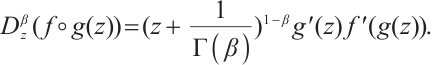
Fractional derivatives, as global operators in generalized fractional calculus, combine differentiation with convolution integrals to capture non-locality and memory effects. In contrast, the beta derivative, derived from traditional integer-order derivatives with an added nonlinear term, lacks the characteristics of a global operator. While fractional derivatives inherently describe long-range dependencies and historical effects, the beta derivative is more localized, making it suitable for scenarios where global properties are less relevant.
Let  is specified as a function of all non-negative
  with the
  derivative[38-39], hence
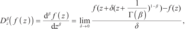
 in which
  is the Gamma function.
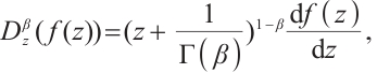
Some effective properties of above definition[38-41] are included
By using the knowledge of fractional derivative and the Bernoulli  -expansion method, the closed-form solutions of FDR equation can be obtianed conveniently. Seeking closed form solutions of FDR equation is facilitated by exerting the Bernoulli
  -expansion method which is presented according to the following steps.
Consider the space-time NFDE as follows
 (2)
(2)
in which  is the polynomial of unknown function
  and its fractional derivatives.
Step 1 Insert the transformation
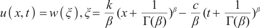 (3)
(3)
into space-time NFDE (2) to yield
 (4)
(4)
where  are constants that may relate to wave speed, and
  is the polynomial of
  along with its derivatives.
Step 2 Assume that (4) has the following solution
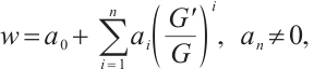 (5)
(5)
where  for
for are constants.
To describe Bernoulli  -expansion method, the following Bernoulli equation for
  needs to be introduced:
 (6)
(6)
where  and
and  are constants
  can be specified later.
Step 3 In Eq. (4), by balancing the highest order derivative of w and highest order nonlinear term, we obtian integer  . By replacing (5) and (6) into (4), a system of algebra equations will be acquired through the gathering of G with the same order.
Step 4 Inserting the results of above steps into (5) and using the following general solutions of (6):
 (7)
(7)
provided  is an integral constant, we achieve closed form solutions of Eq. (2).
2 Applications to the Density-Independent FDR Equation
By inserting transformation (3) in Eq.(1), we can derive an ordinary differential equation as below
 (8)
(8)
By balancing between  and
and  in Eq. (8),
  can be determined for (5), which yields the solution of
  as follows:
 (9)
(9)
where  is satisfied with (6). To gain the meaningful solutions, displacing (9) along with (6) into (8), with collecting coefficients of the same order of
  to zero, a system of algebraic equations is attained as follows:
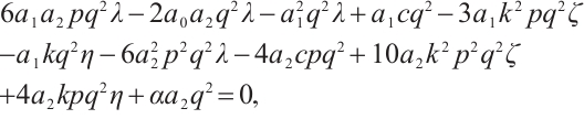
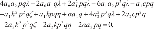
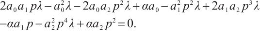
The begotten results for coefficients are as below.
Family 1: 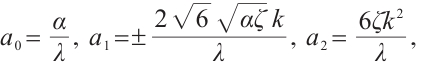
Replacing these results into (9) and by using the definition of  , the following solutions are extracted for (1):
 (10)
(10)
 (11)
(11)
where  and
and  are arbitrary constants and
  , respectively.
Dynamic behaviors of  and
and  are displayed in Figs.1 and 2, by considering
  and
and  , for different values of
 and
and 
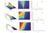 |
Fig. 1 Closed form solution  of Eq. (1), where panels (a1-a3) correspond to of Eq. (1), where panels (a1-a3) correspond to  , (b1-b3) to , (b1-b3) to  and (c1-c3) to and (c1-c3) to 
|
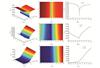 |
Fig. 2 Closed form solution  of Eq. (1), where panels (a1-a3) correspond to of Eq. (1), where panels (a1-a3) correspond to  , (b1-b3) to , (b1-b3) to  and (c1-c3) to and (c1-c3) to 
|
Family 2: 
Replacing these results into (9) and by using the definition of  , the following solutions are extracted for (1):
 (12)
(12)
 (13)
(13)
where  and
and  are constants and
  , respectively.
Figures 3 and 4 are displayed for exact solution of  and
and  , respectively, in 3D, contour map and line plots by setting
  , for different values of
  ,
,  and
and  .
.
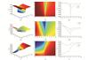 |
Fig. 3 Closed form solution  of Eq. (1), where panels (a1-a3) correspond to of Eq. (1), where panels (a1-a3) correspond to  , (b1-b3) to , (b1-b3) to  and (c1-c3) to and (c1-c3) to 
|
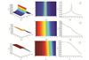 |
Fig. 4 Closed form solution  of Eq. (1), where panels (a1-a3) correspond to of Eq. (1), where panels (a1-a3) correspond to  , (b1-b3) to , (b1-b3) to  and (c1-c3) to and (c1-c3) to 
|
Family 3: 
Replacing these results into (9) and by using the definition of  , the following solutions are extracted for Eq. (1),
 (14)
(14)
 (15)
(15)
where  and
and  are arbitrary constants and
  , respectively.
Figures 5 and 6 conclude 3D, contour map and line plots of  and
and  , respectively, by setting
  for different values of
  ,
,  and
and  .
.
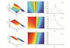 |
Fig. 5 Closed form solution  of Eq. (1), where panels (a1-a3) correspond to of Eq. (1), where panels (a1-a3) correspond to  , (b1-b3) to , (b1-b3) to  and (c1-c3) to and (c1-c3) to 
|
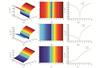 |
Fig. 6 Closed form solution  of Eq. (1), where panels (a1-a3) correspond to of Eq. (1), where panels (a1-a3) correspond to  , (b1-b3) to , (b1-b3) to  and (c1-c3) to and (c1-c3) to 
|
Family 4: 

Replacing these results into (9) and by using the definition of  , the following solutions are extracted for Eq. (1),
 (16)
(16)
 (17)
(17)
where  and
and  are constants and
  , respectively.
We show 3D, contour map and line plots of  and
and  in Fig. 7 and Fig. 8, respectively, by exerting
  for different values of (a1-a3)
 , (b1-b3)
  and (c1-c3)
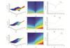 |
Fig. 7 Closed form solution  of Eq. (1), where panels (a1-a3) correspond to of Eq. (1), where panels (a1-a3) correspond to  , (b1-b3) to , (b1-b3) to  and (c1-c3) to and (c1-c3) to 
|
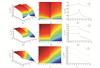 |
Fig. 8 Closed form solution  of Eq. (1), where panels (a1-a3) correspond to of Eq. (1), where panels (a1-a3) correspond to  , (b1-b3) to , (b1-b3) to  and (c1-c3) to and (c1-c3) to 
|
We find that the parameter  mainly affects the negative part of
  in Figs. 1, 2, 6, 7 and 8, while in Figs. 3, 4, 5,
  influences the entire region. As shown in the figures, an increase in
  results in a decrease of the solutions in the negative half-plane of
  . Moreover, for two solutions within a given family, the trends in the changes of convexity and concavity oppose each other as
  increases. These observations may be related to the inherent properties of Eq. (1). Additionally, the simulations reveal that the solutions
  exhibit bright soliton dynamic in certain cases, while
  show dark soliton dynamic. The different behaviors of the solution may be useful to the population prediction, showing the peek and valley of the population.
3 Conclusion
In this article, due to the use of wave transformation which contains  function, the complexity of FDE could be reduced to ordinary differential equation. We find eight new rational exponent solutions to Eq. (1) with Bernoulli
  -expansion method. We derived bright and dark soliton solutions of density-independent FDR equation with quadratic nonlinearity by use of the Bernoulli
  -expansion method. Moreover, 3D, contour map and line plots were demonstrated to show the effect of different values of the derivative of order
  on wave structures. The influences of parameter
  is extracted by comparing the simulations figures. Parameter
  largely affects the negative region of
  . Additionally,
  influences the trends in the convexity and concavity. By these results, we predict that the Bernoulli
  -expansion method can be satisfied enormous range of fractional differential equations.
Although we have obtained numerous results regarding the solutions, the real-world applications of this model still require further investigation.
References
- Liu J G, Ye Q. Stripe solitons and lump solutions for a generalized Kadomtsev-Petviashvili equation with variable coefficients in fluid mechanics[J]. Nonlinear Dynamics, 2019, 96(1): 23-29. [Google Scholar]
- Liu J G, Zhu W H, He Y. Variable-coefficient symbolic computation approach for finding multiple rogue wave solutions of nonlinear system with variable coefficients[J]. Zeitschrift Für Angewandte Mathematik Und Physik, 2021, 72(4): 154. [Google Scholar]
- Ozkan E M. New exact solutions of some important nonlinear fractional partial differential equations with beta derivative[J]. Fractal and Fractional, 2022, 6(3): 173. [Google Scholar]
- Tang B, He Y N, Wei L L, et al. A generalized fractional sub-equation method for fractional differential equations with variable coefficients[J]. Physics Letters A, 2012, 376(38-39): 2588-2590. [Google Scholar]
- Bekir A, Aksoy E, Cevikel A C. Exact solutions of nonlinear time fractional partial differential equations by sub-equation method[J]. Mathematical Methods in the Applied Sciences, 2015, 38(13): 2779-2784. [Google Scholar]
- Sooppy Nisar K, Enam Inan I, Inc M, et al. Properties of some higher-dimensional nonlinear Schrödinger equations[J]. Results in Physics, 2021, 31: 105073. [Google Scholar]
- Mirzazadeh M, Eslami M, Biswas A. Solitons and periodic solutions to a couple of fractional nonlinear evolution equations[J]. Pramana, 2014, 82(3): 465-476. [Google Scholar]
- Eslami M, Fathi Vajargah B, Mirzazadeh M, et al. Application of first integral method to fractional partial differential equations[J]. Indian Journal of Physics, 2014, 88(2): 177-184. [Google Scholar]
- Hosseini K, Mirzazadeh M, Baleanu D, et al. The generalized complex Ginzburg-Landau model and its dark and bright soliton solutions[J]. The European Physical Journal Plus, 2021, 136(7): 709. [Google Scholar]
- Hosseini K, Mirzazadeh M, Salahshour S, et al. Specific wave structures of a fifth-order nonlinear water wave equation[J]. Journal of Ocean Engineering and Science, 2022, 7(5): 462-466. [Google Scholar]
- Kaplan M, Bekir A. A novel analytical method for time-fractional differential equations[J]. Optik, 2016, 127(20): 8209-8214. [Google Scholar]
- Hosseini K, Bekir A, Ansari R. Exact solutions of nonlinear conformable time-fractional Boussinesq equations using the exp(-φ(z))-expansion method[J]. Optical and Quantum Electronics, 2017, 49(4): 131. [Google Scholar]
- Khan K, Ali Akbar M, Koppelaar H. Study of coupled nonlinear partial differential equations for finding exact analytical solutions[J]. Royal Society Open Science, 2015, 2(7): 140406. [Google Scholar]
- Zafar A, Raheel M, Asif M, et al. Some novel integration techniques to explore the conformable M-fractional Schrödinger-Hirota equation[J]. Journal of Ocean Engineering and Science, 2022, 7(4): 337-344. [Google Scholar]
- Nisar K S, Ali K K, Inc M, et al. New solutions for the generalized resonant nonlinear Schrödinger equation[J]. Results in Physics, 2022, 33: 105153. [Google Scholar]
- Sooppy Nisar K, Inan I E, Yepez-Martinez H, et al. Some new type optical and the other soliton solutions of coupled nonlinear Hirota equation[J]. Results in Physics, 2022, 35: 105388. [Google Scholar]
- Tariq H, Akram G. New approach for exact solutions of time fractional Cahn-Allen equation and time fractional Phi-4 equation[J]. Physica A: Statistical Mechanics and Its Applications, 2017, 473: 352-362. [Google Scholar]
- Raslan K R, Ali K K, Shallal M A. The modified extended tanh method with the Riccati equation for solving the space-time fractional EW and MEW equations[J]. Chaos, Solitons & Fractals, 2017, 103: 404-409. [Google Scholar]
-
Hu H C, Li X D. New interaction solutions of the similarity reduction for the integrable
 -dimensional Boussinesq equation[J]. International Journal of Modern Physics B, 2022, 36(1): 2250001.
[Google Scholar]
-dimensional Boussinesq equation[J]. International Journal of Modern Physics B, 2022, 36(1): 2250001.
[Google Scholar]
- Kumar D, Hosseini K, Kaabar M K A, et al. On some novel solution solutions to the generalized Schrödinger-Boussinesq equations for the interaction between complex short wave and real long wave envelope[J]. Journal of Ocean Engineering and Science, 2022, 7(4): 353-362. [Google Scholar]
- Khater M M A, Jhangeer A, Rezazadeh H, et al. Propagation of new dynamics of longitudinal bud equation among a magneto-electro-elastic round rod[J]. Modern Physics Letters B, 2021, 35(35): 2150381. [Google Scholar]
- Kaplan, M, Bekir, A, Akbulut, A, et al. The modified simple equation method for nonlinear fractional differential equations. Romanian Journal of Physics, 2015, 60(9-10):1374. [Google Scholar]
- Kaplan M, Koparan M, Bekir A. Regarding on the exact solutions for the nonlinear fractional differential equations[J]. Open Physics, 2016, 14(1): 478-482. [Google Scholar]
- Rahman Z, Abdeljabbar A, Harun-Or-Roshid, et al. Novel precise solitary wave solutions of two time fractional nonlinear evolution models via the MSE scheme[J]. Fractal and Fractional, 2022, 6(8): 444. [Google Scholar]
- Gu Y Y, Yuan W J, Aminakbari N, et al. Meromorphic solutions of some algebraic differential equations related Painlevé equation IV and its applications[J]. Mathematical Methods in the Applied Sciences, 2018, 41(10): 3832-3840. [Google Scholar]
- Gu Y Y, Wu C F, Yao X, et al. Characterizations of all real solutions for the KdV equation and WR[J]. Applied Mathematics Letters, 2020, 107: 106446. [Google Scholar]
- Gu Y Y, Liao L W. Closed form solutions of Gerdjikov–Ivanov equation in nonlinear fiber optics involving the beta derivatives[J]. International Journal of Modern Physics B, 2022, 36(19): 2250116. [Google Scholar]
- Liu J G, Zhu W H, Wu Y K, et al. Application of multivariate bilinear neural network method to fractional partial differential equations[J]. Results in Physics, 2023, 47: 106341. [Google Scholar]
- Uddin M H, Akbar M A, Khan M A, et al. Close form solutions of the fractional generalized reaction duffing model and the density dependent fractional diffusion reaction equation[J]. Applied and Computational Mathematics, 2017, 6(4): 177-184. [Google Scholar]
- Hosseini K, Mayeli P, Bekir A, et al. Density-dependent conformable space-time fractional diffusion-reaction equation and its exact solutions[J]. Communications in Theoretical Physics, 2018, 69(1): 1. [Google Scholar]
-
Rezazadeh H, Manafian J, Khodadad F S, et al. Traveling wave solutions for density-dependent conformable fractional diffusion-reaction equation by the first integral method and the improved
 ))-expansion method[J]. Optical and Quantum Electronics, 2018, 50: 1-15.
[CrossRef]
[Google Scholar]
))-expansion method[J]. Optical and Quantum Electronics, 2018, 50: 1-15.
[CrossRef]
[Google Scholar]
-
Sene N, Fall A N. Homotopy perturbation
 -Laplace transform method and its application to the fractional diffusion equation and the fractional diffusion-reaction equation[J]. Fractal and Fractional, 2019, 3(2): 14.
[Google Scholar]
-Laplace transform method and its application to the fractional diffusion equation and the fractional diffusion-reaction equation[J]. Fractal and Fractional, 2019, 3(2): 14.
[Google Scholar]
-
Wang M L, Li X Z, Zhang J L. The (
 )-expansion method and travelling wave solutions of nonlinear evolution equations in mathematical physics[J]. Physics Letters A, 2008, 372(4): 417-423.
[Google Scholar]
)-expansion method and travelling wave solutions of nonlinear evolution equations in mathematical physics[J]. Physics Letters A, 2008, 372(4): 417-423.
[Google Scholar]
- Kumar R, Kaushal R S, Prasad A. Some new solitary and travelling wave solutions of certain nonlinear diffusion-reaction equations using auxiliary equation method[J]. Physics Letters A, 2008, 372(19): 3395-3399. [Google Scholar]
- Kumar D, Seadawy A R, Joardar A K. Modified Kudryashov method via new exact solutions for some conformable fractional differential equations arising in mathematical biology[J]. Chinese Journal of Physics, 2018, 56(1): 75-85. [Google Scholar]
- Murray J D. Mathematical Biology[M]. Heidelberg: Springer-Verlag, 1993. [Google Scholar]
- Kenkre V M, Kuperman M N. Applicability of the Fisher equation to bacterial population dynamics[J]. Physical Review E, 2003, 67(5): 051921. [Google Scholar]
- Atangana A, Doungmo Goufo E F. Extension of matched asymptotic method to fractional boundary layers problems[J]. Mathematical Problems in Engineering, 2014, 2014: 107535. [Google Scholar]
- Atangana A, Alqahtani R. Modelling the spread of river blindness disease via the caputo fractional derivative and the beta-derivative[J]. Entropy, 2016, 18(2): 40. [Google Scholar]
- Hosseini K, Mirzazadeh M, Gómez-Aguilar J F. Soliton solutions of the Sasa-Satsuma equation in the monomode optical fibers including the beta-derivatives[J]. Optik, 2020, 224: 165425. [Google Scholar]
-
Hosseini K, Kaur L, Mirzazadeh M, et al. 1-Soliton solutions of the
 -dimensional Heisenberg ferromagnetic spin chain model with the beta time derivative[J]. Optical and Quantum Electronics, 2021, 53(2): 125.
[Google Scholar]
-dimensional Heisenberg ferromagnetic spin chain model with the beta time derivative[J]. Optical and Quantum Electronics, 2021, 53(2): 125.
[Google Scholar]
All Figures
|
Fig. 1 Closed form solution of Eq. (1), where panels (a1-a3) correspond to , (b1-b3) to and (c1-c3) to
|
| In the text | |
|
Fig. 2 Closed form solution of Eq. (1), where panels (a1-a3) correspond to , (b1-b3) to and (c1-c3) to
|
| In the text | |
|
Fig. 3 Closed form solution of Eq. (1), where panels (a1-a3) correspond to , (b1-b3) to and (c1-c3) to
|
| In the text | |
|
Fig. 4 Closed form solution of Eq. (1), where panels (a1-a3) correspond to , (b1-b3) to and (c1-c3) to
|
| In the text | |
|
Fig. 5 Closed form solution of Eq. (1), where panels (a1-a3) correspond to , (b1-b3) to and (c1-c3) to
|
| In the text | |
|
Fig. 6 Closed form solution of Eq. (1), where panels (a1-a3) correspond to , (b1-b3) to and (c1-c3) to
|
| In the text | |
|
Fig. 7 Closed form solution of Eq. (1), where panels (a1-a3) correspond to , (b1-b3) to and (c1-c3) to
|
| In the text | |
|
Fig. 8 Closed form solution of Eq. (1), where panels (a1-a3) correspond to , (b1-b3) to and (c1-c3) to
|
| In the text | |
Current usage metrics show cumulative count of Article Views (full-text article views including HTML views, PDF and ePub downloads, according to the available data) and Abstracts Views on Vision4Press platform.
Data correspond to usage on the plateform after 2015. The current usage metrics is available 48-96 hours after online publication and is updated daily on week days.
Initial download of the metrics may take a while.