© Wuhan University 2025

0 Introduction

Chaos exists in all aspects of nature, such as chemical engineering^[1-2], mechanical engineering^[3-4], and biological engineering^[5-6]. Chaos is a unique motion state of some nonlinear systems, with unstable attractors. Namely, the motion state of the nonlinear dynamic system is unstable and then bifurcates, and finally enters into the chaotic state. In recent decades, chaos has been one of the important contents of nonlinear scientific research.

The dynamic analysis of new discrete chaotic systems has become one of the research directions in nonlinear scientific research^[7-12]. By conducting dynamic analysis on discrete chaotic systems, the periodic and chaotic solutions of the system are obtained, which enter the chaotic system through a doubling bifurcation process^[7-9]. Nategh et al^[8] analyzed the dynamic of delayed discrete chaotic systems with delay. Time delay appears in an additive form. By analyzing the dynamics of time-delay discrete chaotic systems, it is found that the system is neutral to bounded delays and has attractive fixed points in both additive and non-additive forms. Chen et al^[10] analyzed a predator-prey discrete chaotic system. Using the new paradigm, central manifold theorem, and bifurcation theory of discrete singular systems, the occurrence of flipping bifurcation and Neimark Sacker bifurcation in the system was analyzed. This discrete chaotic system has rich dynamic characteristics. Dai et al^[12] generated a discrete chaotic system using fractal transformation. The dynamic characteristics of this discrete chaotic system were analyzed from the aspects of bifurcation, complexity, and spectral distribution characteristics. The discrete chaotic system was verified with circuits. These studies indicate that discrete chaotic systems have rich nonlinear dynamic characteristics and can be applied in engineering, such as biotechnology^[10], communication encryption^[12-13], etc.

The chaos control of discrete chaotic systems is another important direction in nonlinear scientific research. The main contents of chaos control in discrete chaotic systems include synchronization control^[14-16], bifurcation control^[17-18], and others^[19-21]. Yong et al^[14] proposed a control method based on the backstepping design of three controllers to study the function projection synchronization of discrete-time chaotic systems with uncertain parameters. Zhang et al^[15] used a pulse controller to perform lag synchronization control on a discrete chaotic system, obtaining sufficient conditions for synchronization between the driving system and the response system. Zhang et al^[17] analyzed and controlled the symmetry-breaking bifurcation of cubic discrete chaos, and obtained the cause of the symmetry-breaking bifurcation. A controller was set for the system to make the symmetry-breaking bifurcation disappear and the period-doubling bifurcation recover. Din^[19] studied a discrete-time predator-prey system and analyzed its dynamic characteristics, such as boundedness, existence, and bifurcation. The feedback control method was used to delay the generation of bifurcation and avoid chaos. Tang et al^[20] used neural network control methods to control chaos in a class of discrete chaotic systems. This method can generate the optimal control input and effectively make the system bounded. These studies rarely involve the control of intermittent chaos and period-doubling bifurcation in discrete chaotic systems, and even less so for two-peak discrete chaotic systems. In this paper, the dynamic characteristics of a two-peak discrete chaotic system are analyzed to verify the causes of intermittent chaos. Linear and nonlinear state feedback controllers are set up for the discrete chaotic system to control the chaos, to delay the generation of bifurcations, and to expand the stability range of the system. The goal of chaos control is achieved.

The paper is arranged as follows: In Section 1, the dynamic characteristics of the two-peak discrete chaotic system are analyzed to obtain the system motion process. In Section 2, the conditions of intermittent chaos are analyzed, and the motion process of intermittent chaos is expounded. In Section 3, linear controllers and nonlinear controllers are set to the system to delay or eliminate chaos. Finally, Section 4 summarizes this paper.

1 Two-Peak Discrete Chaotic System

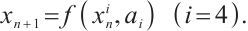
When a discrete chaotic system exhibits two chaotic states, this discrete chaotic system is called a two-peak discrete chaotic system. Two-peak discrete chaotic systems are generally composed of high-power chaotic systems, and their coefficients can be determined by specific conditions. The nonlinear dynamic model of a two-peak discrete chaotic system is as follows:

$x_{n+\mathrm{1}}=f\left(x_n^i,a_i\right)\left(i=\mathrm{4}\right).$(1)

We can write the general iteration of (1) as follows:

$x_{n+\mathrm{1}}=-\mathrm{12.5}a{x}^{\mathrm{4}}+\mathrm{25}a{x}^{\mathrm{3}}-\mathrm{12.5}(a+\mathrm{1})x^{\mathrm{2}}+\mathrm{12.5}x,$(2)

where $a>\mathrm{0}$.

By taking the system parameter $a$ as the bifurcation parameter, bifurcation can be obtained by numerical calculation of system formula (2) when the initial value $x_{\mathrm{0}}=\mathrm{0.6}$, as shown in Fig. 1.

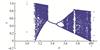Fig. 1 Bifurcation diagram

From Fig. 1, we can see the system state movement process. The system starts from a chaotic state, goes through intermittent chaos, a stable state, period-doubling bifurcation, and then goes through a transient stable state, and finally enters an intermittent chaotic state again. The two-peak discrete chaotic system is that within the range of the system parameters, the system appears the secondary chaotic state in the process of motion. This bifurcation diagram just verifies this definition.

To better understand the nonlinear dynamic behavior of two-peak discrete chaotic systems, we draw the Lyapunov exponent spectrum of two-peak discrete chaotic systems, as shown in Fig. 2.

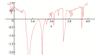Fig. 2 Lyapunov exponents of the system (2)

It can be seen from Fig. 2 that the shape of the Lyapunov exponent spectrum changes with the change of system parameter $a$. When $a\in (\mathrm{0},\mathrm{3.25})$, the system (2) is in intermittent chaos. There are periodic windows in the process. When $a\in (\mathrm{3.25},\mathrm{3.467})$, the system enters a stable state and is in one period. When $a=\mathrm{3.467}$, the system enters the period-doubling bifurcation state, one period is divided into two periods. When $a\in (\mathrm{3.467},\mathrm{3.578})$, the system continues to be in the period-doubling bifurcation state, which is divided into four periods from two periods and eight periods from four periods. When $a\in \left(\mathrm{3.578,4}\right)$, the system enters a chaotic state.

The motion process of the two-peak discrete chaotic system (2) can also be seen from the waveform of the system. The system from an unstable state to a stable state, then to a stable periodic solution, and finally to an unstable state. The waveform is shown in Fig. 3.

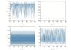Fig. 3 Waveform diagram

2 Intermittent Chaos

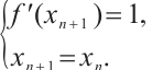
Period doubling bifurcation is one of the ways in which the system enters chaos. When the system exhibits chaotic formation, the system is unstable and lacks periodic solutions. The system is in a chaotic state. The critical condition for the system to generate intermittent chaos is the system parameter value when the system angular line is tangent to the two-peak discrete chaotic system (2). According to the reasoning of the tangent equation in equation (2), when the tangent equation passes through the origin and the slope $k=\mathrm{1}\left(\theta =\mathrm{45}°\right)$, the chaotic system is in a critical state, and the tangent point is a fixed point. At this time, the system parameter $a$ value is a critical condition. From the condition of the fixed point, we get

$f^{\text{'}}\left(x_n^i,a_i\right)=\mathrm{1}.$(3)

When the two-peak discrete chaotic system (2) is tangent to the angular line, there is $x_{n+\mathrm{1}}=x_n$. Namely,

$-\mathrm{12.5}a{x}^{\mathrm{3}}+\mathrm{25}a{x}^{\mathrm{2}}-\mathrm{12.5}(a+\mathrm{1})x+\mathrm{11.5}=\mathrm{0}.$(4)

By solving equations (3) and (4), we can get the iterative algebraic value $x$ and system parameters of the chaotic system (2) when it is tangent to the diagonal line. The quadratic function relationship of iteration value $x$ and system parameters $a$ is:

$x_{\mathrm{1,2}}=\frac{\mathrm{1}}{\mathrm{2}a}\left(\mathrm{1}+a\mp \sqrt[]{a-\mathrm{3.208}}\sqrt[]{a-\mathrm{0.3117}}\right)$(5)

We substitute the two conditions of equation (5) back to equation (4) to obtain the critical values of a two-peak discrete chaotic system. The critical values are $a_{\mathrm{1}}=\mathrm{3.32}$ and $a_{\mathrm{2}}=\mathrm{3.764}$. The calculated critical values are the same as the occurrence of intermittent chaos in the bifurcation diagram in Fig. 1.

Next, we analyze the dynamic characteristics of intermittent chaos. The local bifurcation of the system (2) is shown in Fig. 4.

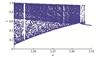Fig. 4 Local bifurcation diagram

In Fig. 4, the evacuation area with fewer values in the chaotic area is an intermittent chaotic process. In the process of numerical iteration, the number of iterations around the fixed point is far greater than that of the intermittent chaotic process, then there are two chaotic regions: evacuation and dense. It can be seen from the figure that when the system parameter $a$ gradually increases, the evacuation area gradually decreases, the numerical range of the intermittent chaotic process gradually narrows, and the iterative process becomes shorter. This shows that the distance between $f\left(x_n^i,a_i\right)$ and the angular line $\left(\theta =\mathrm{45}°\right)$ is getting closer and closer. Finally, $f\left(x_n^i,a_i\right)$ is tangent to the angular line $\left(\theta =\mathrm{45}°\right)$, and the system changes from intermittent chaos to a stable fixed point.

The local Lyapunov exponents of the system (2) are shown in Fig. 5. From the figure, we can see that there are two chaotic windows in intermittent chaos, which indicates that the process of intermittent chaos also includes chaos and periodic motion. The motion process of the system starts from intermittent chaos to period-doubling bifurcation. Figure 6 shows the fine structure of the window chaotic behavior.

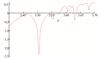Fig. 5 Local Lyapunov exponents

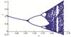Fig. 6 Fine structure of window chaotic behavior

3 Chaos Control

One of the purposes of chaos control is to change the position where chaos occurs so that the position where chaos occurs is delayed or advanced. We set linear controllers and nonlinear controllers for system (2) to change the position of intermittent chaos.

3.1 Linear Controllers

Set linear controllers for the system (2) without changing the system equilibrium point. The controlled system is as follows:

$x_{n+\mathrm{1}}=-\mathrm{12.5}a{x}^{\mathrm{4}}+\mathrm{25}a{x}^{\mathrm{3}}-\mathrm{12.5}(a+\mathrm{1})x^{\mathrm{2}}+\mathrm{12.5}x+k_{\mathrm{1}}x$(6)

where $k_{\mathrm{1}}$ is the control parameter.

According to the critical condition of intermittent chaos, we can get

$\{\begin{array}{l}{f}^{\text{'}}(x_{n+\mathrm{1}})=\mathrm{1},\\ x_{n+\mathrm{1}}=x_n.\end{array}$(7)

Through detailed calculation, we can get the relationship between the system parameter $a$ and the control parameter $k_{\mathrm{1}}$:

$\mathrm{25}a{x}^{\mathrm{3}}-\mathrm{25}(a+\mathrm{1})x^{\mathrm{2}}+\mathrm{34.5}x+\mathrm{3}{k}_{\mathrm{1}}=\mathrm{0}.$(8)

Set $k_{\mathrm{1}}=\mathrm{0.1}$, then $a_{\mathrm{3}}=\mathrm{3.393}$ and $a_{\mathrm{4}}=\mathrm{4.092}$. Similar to the system (2), the positions of intermittent chaos are delayed.

From the bifurcation diagram (Fig. 7) and Lyapunov exponential diagram (Fig. 8) of the system (6), we can see that the dynamic characteristics of the system have changed. The experience time of intermittent chaos of the system becomes shorter, and the critical point from intermittent chaos to a stable state is delayed from 3.32 to 3.39. When $a=\mathrm{3.627}$, the system is divided into two periodic states from one periodic state, and then into four periodic states, until it enters a chaotic state. When $a=\mathrm{3.765}$, the system jumps, and the system goes from chaos to stability. When $a=\mathrm{4.092}$, the system jumps into intermittent chaos. Under the effect of the control parameter $k_{\mathrm{1}}$, intermittent chaos becomes narrower with the increase of system parameter $a$.

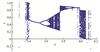Fig. 7 Bifurcation diagram of the system (6) when ${\mathit{k}}_{\mathrm{1}}=\mathrm{0.1}$

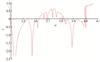Fig. 8 Lyapunov exponents of the system (6) when ${\mathit{k}}_{\mathrm{1}}=\mathrm{0.1}$

Set $k_{\mathrm{1}}=\mathrm{0.5}$, the intermittent chaos of the system (6) is disappeared. The motion process of the system is in a stable state. After the period-doubling bifurcation, it finally enters a chaotic state, as shown in Fig. 9.

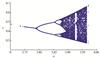Fig. 9 Bifurcation diagram of the system (6) when ${\mathit{k}}_{\mathrm{1}}=\mathrm{0.5}$

3.2 Nonlinear Controller

The wavelet function is an important nonlinear controller. Wavelet functions have oscillatory properties. As the independent variable continues to extend in the positive and negative directions, the wavelet function rapidly decays. As a controller for chaotic systems, wavelet functions can suppress the chaotic behavior of the system. Due to the non or thogonality and scale function of the Metican wavelet function, it has good localization properties in both the time and frequency domains, while satisfying the requirement of zero infinite integration on all real number intervals. Therefore, the metric wavelet function is chosen as the nonlinear controller of the system.

The mathematical expression for the metric wavelet function is

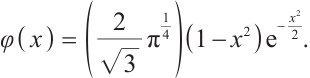$\phi \left(x\right)=\left(\frac{\mathrm{2}}{\sqrt[]{\mathrm{3}}}{\mathrm{\pi }}^{\frac{\mathrm{1}}{\mathrm{4}}}\right)\left(\mathrm{1}-x^{\mathrm{2}}\right){\mathrm{e}}^{-\frac{x^{\mathrm{2}}}{\mathrm{2}}}.$(9)

To obtain more control results, the coefficients of the wavelet function are set to the gain coefficient $k_{\mathrm{2}}$. By adjusting the value of the gain coefficient $k_{\mathrm{2}}$, chaos control of the system (1) is achieved.

The controlled system is as follows:

$x_{n+\mathrm{1}}=\left(\mathrm{12.5}x-\mathrm{12.5}(a+\mathrm{1})x^{\mathrm{2}}+\mathrm{25}a{x}^{\mathrm{3}}-\mathrm{12.5}a{x}^{\mathrm{4}}\right)k_{\mathrm{2}}\left(\mathrm{1}-x^{\mathrm{2}}\right){\mathrm{e}}^{-\frac{x^{\mathrm{2}}}{\mathrm{2}}}$(10)

where $k_{\mathrm{2}}$ is the control parameter.

According to equation (7), the relationship between the system parameter $a$ and the control parameter $k_{\mathrm{2}}$ is obtained.

$k_{\mathrm{2}}{\mathrm{e}}^{-\frac{x^{\mathrm{2}}}{\mathrm{2}}}[\mathrm{12.5}-(\mathrm{25}+\mathrm{25}a)x+(\mathrm{75}a-\mathrm{50})x^{\mathrm{2}}+(\mathrm{12.5}a+\mathrm{62.5})x^{\mathrm{3}}+(\mathrm{12.5}-\mathrm{150}a)x^{\mathrm{4}}+(\mathrm{75}a-\mathrm{12.5})x^{\mathrm{5}}+\mathrm{25}a{x}^{\mathrm{6}}-\mathrm{12.5}a{x}^{\mathrm{7}}]=\mathrm{1}$(11)

Set $k_{\mathrm{2}}=\mathrm{0.2}$, the bifurcation diagram and Lyapunov exponential diagram of the system are shown in Fig. 10 and Fig. 11.

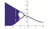Fig.10 Bifurcation diagram of the system (10) when ${\mathit{k}}_{\mathrm{2}}=\mathrm{0.2}$

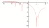Fig.11 Lyapunov exponents of the system (10) when ${\mathit{k}}_{\mathrm{2}}=\mathrm{0.2}$

From Fig. 10 and Fig. 11, it can be seen that the intermittent chaos of the system (10) is disappeared. The controlled system only has one process of transitioning from period-doubling bifurcation to chaos. The system has two chaotic processes, only one of which enters chaos through period-doubling bifurcation. When $a>-\mathrm{0.906}$, the system is in a stable state. When $a=-\mathrm{0.906}$, the system has period-doubling bifurcation. The system is divided into two periodic states from one periodic state, and then into four periodic states, eight periodic states, until enters a chaotic state. Under the action of a nonlinear controller, the system transitions from two complex chaotic processes to a process of transitioning from period-doubling bifurcation to chaos. The direction of the period-doubling bifurcation of the controlled system changes, becoming an inverted bifurcation. The critical value of bifurcation is less than 0, and the occurrence of chaos is delayed, expanding the stability range of the system.

Set $k_{\mathrm{2}}=\mathrm{0.5}$, the system has returned to the state of two chaotic processes, but there has been no occurrence of intermittent chaos. The bifurcation diagram and Lyapunov exponential diagram of the system are shown in Fig. 12 and Fig. 13.

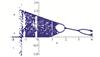Fig.12 Bifurcation diagram of the system (10) when ${\mathit{k}}_{\mathrm{2}}=\mathrm{0.5}$

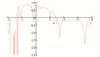Fig.13 Lyapunov exponents of the system (10) when ${\mathit{k}}_{\mathrm{2}}=\mathrm{0.5}$

From Fig. 12 and Fig. 13, it can be seen that the dynamic characteristics of the controlled system (10) are the same as those of the original system (2). Just under the action of the controller, the stability range of the system changes from $\left(\mathrm{3.328,3},\mathrm{46}\right)$ to $\left(\mathrm{1.997,3.007}\right)$. The stable range has been expanded. Meanwhile, the intermittent chaos of the system (10) transforms into a process of period-doubling bifurcation and entering chaos.

From the above analysis, it can be seen that wavelet functions serving as nonlinear controllers for discrete chaotic systems have good convergence. By adjusting the control parameters of the controller, the stable range of the system can be greatly expanded. Meanwhile, this nonlinear controller can transform complex paroxysmal chaotic processes into a simple process of transitioning from multiplicative bifurcation to chaos. The purpose of chaos control is realized.

4 Conclusion

In our work, the dynamic characteristics of a two-peak discrete chaotic system are studied. The conditions and process of intermittent chaos are analyzed. We set linear controller and nonlinear controller to control the chaos of the system and change the dynamic characteristics of the system. By adjusting the value of control parameters, the position of intermittent chaos in the system changes and can be delayed or disappear. Simulation analysis verifies the correctness of the theoretical analysis.

References

All Figures

	Fig. 1 Bifurcation diagram
In the text

	Fig. 2 Lyapunov exponents of the system (2)
In the text

	Fig. 3 Waveform diagram
In the text

	Fig. 4 Local bifurcation diagram
In the text

	Fig. 5 Local Lyapunov exponents
In the text

	Fig. 6 Fine structure of window chaotic behavior
In the text

	Fig. 7 Bifurcation diagram of the system (6) when ${\mathit{k}}_{\mathrm{1}}=\mathrm{0.1}$
In the text

	Fig. 8 Lyapunov exponents of the system (6) when ${\mathit{k}}_{\mathrm{1}}=\mathrm{0.1}$
In the text

	Fig. 9 Bifurcation diagram of the system (6) when ${\mathit{k}}_{\mathrm{1}}=\mathrm{0.5}$
In the text

	Fig.10 Bifurcation diagram of the system (10) when ${\mathit{k}}_{\mathrm{2}}=\mathrm{0.2}$
In the text

	Fig.11 Lyapunov exponents of the system (10) when ${\mathit{k}}_{\mathrm{2}}=\mathrm{0.2}$
In the text

	Fig.12 Bifurcation diagram of the system (10) when ${\mathit{k}}_{\mathrm{2}}=\mathrm{0.5}$
In the text

	Fig.13 Lyapunov exponents of the system (10) when ${\mathit{k}}_{\mathrm{2}}=\mathrm{0.5}$
In the text

References

- Harmon Ray W, Villa C M. Nonlinear dynamics found in polymerization processes: A review[J]. Chemical Engineering Science, 2000, 55(2): 275-290. [Google Scholar]
- Wu X G, Kapral R. Internal fluctuations and deterministic chemical chaos[J]. Physical Review Letters, 1993, 70(13): 1940-1943. [Google Scholar]
- Huang K, Cheng Z B, Xiong Y S, et al. Bifurcation and chaos analysis of a spur gear pair system with fractal gear backlash[J]. Chaos, Solitons & Fractals, 2021, 142: 110387. [Google Scholar]
- Liu S X, Hu A J, Zhang Y, et al. Nonlinear dynamics analysis of a multistage planetary gear transmission system[J]. International Journal of Bifurcation and Chaos, 2022, 32(7): 2250096. [Google Scholar]
- Sen M, Srinivasu P D N, Banerjee M. Global dynamics of an additional food provided predator-prey system with constant harvest in predators[J]. Applied Mathematics and Computation, 2015, 250: 193-211. [Google Scholar]
- Zhao H Y, Huang X X, Zhang X B. Hopf bifurcation and harvesting control of a bioeconomic plankton model with delay and diffusion terms[J]. Physica A: Statistical Mechanics and Its Applications, 2015, 421: 300-315. [Google Scholar]
- Lu J N, Wu X Q, Lü J H, et al. A new discrete chaotic system with rational fraction and its dynamical behaviors[J]. Chaos, Solitons & Fractals, 2004, 22(2): 311-319. [Google Scholar]
- Nategh M, Baleanu D, Taghizadeh E, et al. Almost local stability in discrete delayed chaotic systems[J]. Nonlinear Dynamics, 2017, 89(4): 2393-2402. [Google Scholar]
- Jiang H B, Li T, Zeng X L, et al. Bifurcation analysis of the logistic map via two periodic impulsive forces[J]. Chinese Physics B, 2014, 23(1): 116-122(Ch). [Google Scholar]
- Chen B S, Chen J J. Bifurcation and chaotic behavior of a discrete singular biological economic system[J]. Applied Mathematics and Computation, 2012, 219(5): 2371-2386. [Google Scholar]
- Sokolov S, Zhilenkov A, Chernyi S, et al. Dynamics models of synchronized piecewise linear discrete chaotic systems of high order[J]. Symmetry, 2019, 11(2): 236. [Google Scholar]
- Dai S Q, Sun K H, Ai W, et al. Novel discrete chaotic system via fractal transformation and its DSP implementation[J]. Modern Physics Letters B, 2020, 34(Supp01): 2050429. [Google Scholar]
- Wang C F, Fan C L, Ding Q. Constructing discrete chaotic systems with positive Lyapunov exponents[J]. International Journal of Bifurcation and Chaos, 2018, 28(7): 1850084. [Google Scholar]
- Yong C, Xin L. Function projective synchronization in discrete-time chaotic system with uncertain parameters[J]. Communications in Theoretical Physics, 2009, 51(3): 470-474. [Google Scholar]
- Zhang L P, Jiang H B, Bi Q S. Reliable impulsive lag synchronization for a class of nonlinear discrete chaotic systems[J]. Nonlinear Dynamics, 2010, 59(4): 529-534. [Google Scholar]
- Ju H P. A new approach to synchronization of discrete-time chaotic systems[J]. Journal of the Physical Society of Japan, 2007, 76(9): 093002. [Google Scholar]
- Zhang L, Han Q. Symmetry breaking bifurcation analysis and control of a cubic discrete chaotic system[J]. The European Physical Journal Special Topics, 2022, 231(11): 2125-2131. [Google Scholar]
- Zhang L, Tang J S, Ouyang K J. Anti-control of period doubling bifurcation for a variable substitution model of Logistic map[J]. Optik, 2017, 130: 1327-1332. [Google Scholar]
- Din Q. Complexity and chaos control in a discrete-time prey-predator model[J]. Communications in Nonlinear Science and Numerical Simulation, 2017, 49: 113-134. [Google Scholar]
- Tang L, Gao Y, Liu Y J. Adaptive near optimal neural control for a class of discrete-time chaotic system[J]. Neural Computing and Applications, 2014, 25(5): 1111-1117. [Google Scholar]
- Ouannas A. A new generalized-type of synchronization for discrete-time chaotic dynamical systems[J]. Journal of Computational and Nonlinear Dynamics, 2015, 10(6): 061019. [Google Scholar]